Nearest Neighbors
Contents
Nearest Neighbors
Given a point cloud, or data set \(X\), and a distance \(d\), a common computation is to find the nearest neighbors of a target point \(x\), meaning points \(x_i \in X\) which are closest to \(x\) as measured by the distance \(d\).
Nearest neighbor queries typically come in two flavors:
Find the
knearest neighbors to a pointxin a data setXFind all points within distance
rfrom a pointxin a data setX
There is an easy solution to both these problems, which is to do a brute-force computation
Brute Force Solution
import numpy as np
import matplotlib.pyplot as plt
import scipy as sp
import scipy.spatial
import scipy.spatial.distance as distance
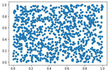
n = 1000
d = 2
X = np.random.rand(n,d)
plt.scatter(X[:,0], X[:,1])
plt.show()
def knn(x, X, k, **kwargs):
    """
    find indices of k-nearest neighbors of x in X
    """
    d = distance.cdist(x.reshape(1,-1), X, **kwargs).flatten()
    return np.argpartition(d, k)[:k]
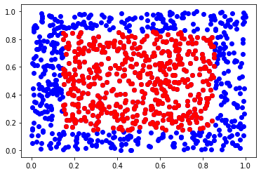
x = np.array([[0.5,0.5]])

inds = knn(x, X, 50)
plt.scatter(X[:,0], X[:,1], c='b')
plt.scatter(X[inds,0], X[inds,1], c='r')
plt.show()

def rnn(x, X, r, **kwargs):
    """
    find r-nearest neighbors of x in X
    """
    d = distance.cdist(x.reshape(1,-1), X, **kwargs).flatten()
    return np.where(d<r)[0]
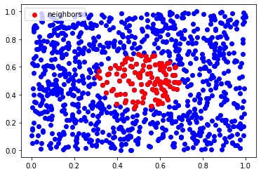
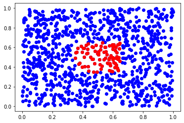
inds = rnn(x, X, 0.2)
plt.scatter(X[:,0], X[:,1], c='b')
plt.scatter(X[inds,0], X[inds,1], c='r', label="neighbors")
plt.legend()
plt.show()
KD-trees
One of the issues with a brute force solution is that performing a nearest-neighbor query takes \(O(n)\) time, where \(n\) is the number of points in the data set. This can become a big computational bottleneck for applications where many nearest neighbor queries are necessary (e.g. building a nearest neighbor graph), or speed is important (e.g. database retrieval)
A kd-tree, or k-dimensional tree is a data structure that can speed up nearest neighbor queries considerably. They work by recursively partitioning \(d\)-dimensional data using hyperplanes.
scipy.spatial provides both KDTree (native Python) and cKDTree (C++). Note that these are for computing Euclidean nearest neighbors
from scipy.spatial import KDTree, cKDTree
tree = KDTree(X)
ds, inds =  tree.query(x, 50) # finds 50-th nearest neighbors

plt.scatter(X[:,0], X[:,1], c='b')
plt.scatter(X[inds,0], X[inds,1], c='r')
plt.show()

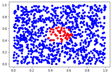
inds = tree.query_ball_point(x, 0.2) # finds neighbors in ball of radius 0.1
inds = inds[0]
plt.scatter(X[:,0], X[:,1], c='b')
plt.scatter(X[inds,0], X[inds,1], c='r')
plt.show()

cKDTrees have the same methods
ctree = scipy.spatial.cKDTree(X)
ds, inds =  ctree.query(x, 50) # finds 50-th nearest neighbors

plt.scatter(X[:,0], X[:,1], c='b')
plt.scatter(X[inds,0], X[inds,1], c='r')
plt.show()
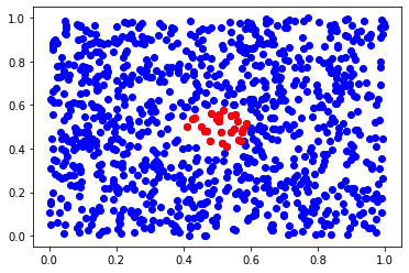
inds = tree.query_ball_point(x, 0.1) # finds neighbors in ball of radius 0.1
inds = inds[0]
plt.scatter(X[:,0], X[:,1], c='b')
plt.scatter(X[inds,0], X[inds,1], c='r')
plt.show()
Performance Comparision
import time

k=50

n = 100000
d = 2
Y = np.random.rand(n,d)

t0 = time.time()
inds = knn(x, Y, 50)
t1 = time.time()
print("brute force: {} sec".format(t1 - t0))

t0 = time.time()
tree = KDTree(Y)
ds, inds =  tree.query(x, 50) # finds 50-th nearest neighbors
t1 = time.time()
print("KDTree: {} sec".format(t1 - t0))

t0 = time.time()
ds, inds =  tree.query(x, 50) # finds 50-th nearest neighbors
t1 = time.time()
print("  extra query: {} sec".format(t1 - t0))

t0 = time.time()
tree = cKDTree(Y)
ds, inds =  tree.query(x, 50) # finds 50-th nearest neighbors
t1 = time.time()
print("cKDTree: {} sec".format(t1 - t0))

t0 = time.time()
ds, inds =  tree.query(x, 50) # finds 50-th nearest neighbors
t1 = time.time()
print("  extra query: {} sec".format(t1 - t0))
brute force: 0.002646207809448242 sec
KDTree: 0.38106298446655273 sec
  extra query: 0.0012862682342529297 sec
cKDTree: 0.049429893493652344 sec
  extra query: 0.00014662742614746094 sec
Ball trees
If you want to do nearest neighbor queries using a metric other than Euclidean, you can use a ball tree. Scikit learn has an implementation in sklearn.neighbors.BallTree.
KDTrees take advantage of some special structure of Euclidean space. Ball Trees just rely on the triangle inequality, and can be used with any metric.
from sklearn.neighbors import BallTree
The list of built-in metrics you can use with BallTree are listed under sklearn.neighbors.DistanceMetric
tree = BallTree(X, metric="minkowski", p=np.inf)
for a k-nearest neighbors query, you can use the query method:
ds, inds = tree.query(x, 500)

plt.scatter(X[:,0], X[:,1], c='b')
plt.scatter(X[inds,0], X[inds,1], c='r')
plt.show()
for r-nearest neighbors, you use query_radius instead of query_ball_point.
inds = tree.query_radius(x, 0.2)
inds = inds[0]

plt.scatter(X[:,0], X[:,1], c='b')
plt.scatter(X[inds,0], X[inds,1], c='r')
plt.show()

tree = BallTree(X, metric='chebyshev')

inds = tree.query_radius(x, 0.15)
inds = inds[0]

plt.scatter(X[:,0], X[:,1], c='b')
plt.scatter(X[inds,0], X[inds,1], c='r')
plt.show()
Exercises
Compare the performance of
KDTree,cKDTree, andBallTreefor doing nearest neighbors queries in the Euclidean metricScikit learn also has a
KDTreeimplementation:sklearn.neighbors.KDTree- how does this compare to the KDTree implementations in scipy?
## Your code here