Distances
Contents
Distances
A common task when dealing with data is computing the distance between two points.
We can use scipy.spatial.distance to compute a variety of distances.
import numpy as np
import scipy.linalg as la
import matplotlib.pyplot as plt
import scipy.spatial.distance as distance
A data set is a collection of observations, each of which may have several features. We’ll consider the situation where the data set is a matrix X, where each row X[i] is an observation. We’ll use n to denote the number of observations and p to denote the number of features, so X is a \(n \times p\) matrix.
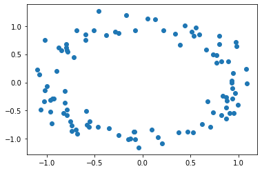
For example, we might sample from a circle (with some gaussian noise)
def sample_circle(n, r=1, sigma=0.1):
    """
    sample n points from a circle of radius r
    add Gaussian noise with variance sigma^2
    """
    X = np.random.randn(n,2)
    X = r * X / np.linalg.norm(X,axis=1).reshape(-1,1)
    return X + sigma * np.random.randn(n,2)

X = sample_circle(100)
plt.scatter(X[:,0], X[:,1])
plt.show()
We might also call a data set a “point cloud”, or a collection of points in some space.
Similarity, Dissimilarity, and Metric
A similarity between two points \(x, y\in X\) is a function \(s: X \times X \to \mathbb{R}\), where \(s\) is larger if \(x,y\) are more similar.
Cosine similarity is an an example of similarity for points in a real vector space. We can define it as \begin{equation} c(x,y) = \frac{x^T y}{|x|_2 |y|_2} \end{equation}
Note \(c(x,x) = 1\), and if \(x,y\) are orthogonal, then \(c(x,y) = 0\).
A dissimilarity between two points \(x,y \in X\) is a function \(d: X \times X \to \mathbb{R}_+\), where \(d\) is smaller if \(x,y\) are more similar. Sometimes, disimilarity functions will be called distances.
Cosine distance is an example of a dissimilarity for points in a real vector space. It is defined as \begin{equation} d(x,y) = 1 - c(x,y) \end{equation} Note \(d(x,x) = 0\), and \(d(x,y) = 1\) if \(x,y\) are orthogonal.
A metric is a disimilarity \(d\) that satisfies the metric axioms
\(d(x,y) = 0\) iff \(x=y\) (identity)
\(d(x,y) = d(y,x)\) (symmetry)
\(d(x,y) \le d(x,z) + d(z,y)\) (triangle inequality)
You are probably most familiar with the Euclidean metric \begin{equation} d(x,y) = |x - y|_2 \end{equation}
Exercise
Write functions for the cosine similarity, cosine distance, and euclidean distance between two numpy arrays treated as vectors.
## Your code here
import numpy as np

cos_sim = lambda x, y : np.dot(x,y) / np.sqrt(np.dot(x,x) * np.dot(y,y))
cos_dis = lambda x, y : 1 - cos_sim(x,y)
euc_dis = lambda x, y : np.linalg.norm(x - y, 2)

x = np.array([1,2,3])
y = np.array([-1,2,3])
print(cos_sim(x,x), cos_dis(x,x), euc_dis(x,x))
print(cos_sim(x,-x), cos_dis(x,-x), euc_dis(x,-x))
print(cos_sim(x,y), cos_dis(x,y), euc_dis(x,y))
1.0 0.0 0.0
-1.0 2.0 7.483314773547883
0.8571428571428571 0.1428571428571429 2.0
X = np.random.randn(100, 3)
X[0].T @ X[0]
2.8389823765022792
X @ X.T
array([[ 2.83898238,  1.16304231, -2.32948147, ..., -3.38312712,
         1.07988589, -0.24763674],
       [ 1.16304231,  8.2530741 , -1.27677546, ...,  0.17204936,
         3.0345908 , -2.39239586],
       [-2.32948147, -1.27677546,  2.23607767, ...,  3.43250478,
        -0.99733681,  0.47330705],
       ...,
       [-3.38312712,  0.17204936,  3.43250478, ...,  6.01431271,
        -0.77625925,  0.24180186],
       [ 1.07988589,  3.0345908 , -0.99733681, ..., -0.77625925,
         1.27487243, -0.85996136],
       [-0.24763674, -2.39239586,  0.47330705, ...,  0.24180186,
        -0.85996136,  0.795015  ]])
x = np.random.randn(1,3)
y = np.random.randn(1,3)
Solution:
# The function for the cosine similarity:
def cosimi(x,y):
    num = x.T @ y
    denum = la.norm(x) * la.norm(y)
    return num/denum

# The functions for the cosine distance:
def cosdis(x,y):
    num = x.T @ y
    denum = la.norm(x) * la.norm(y)
    cosimi = num/denum
    return 1-cosimi

# The function for the euclidean distance:
def euclidis(x,y):
    return la.norm(x-y)
Computing Distances
SciPy provides a variety of functionality for computing distances in scipy.spatial.distance.
x = [1.0, 0.0]
y = [0.0, 1.0]

distance.euclidean(x, y) # sqrt(2)
1.4142135623730951
distance.cosine(x, y)
1.0
the \(L_1\) / Manhattan / City block distance \begin{equation} d(x,y) = |x - y|_1 = \sum_i |x_i - y_i| \end{equation}
distance.cityblock(x, y)
2.0
The \(L_\infty\) / Chebyshev distance \begin{equation} d(x,y) = |x - y|_\infty = \max_i |x_i - y_i| \end{equation}
distance.chebyshev(x, y)
1.0
More generally, the Minkowski distance \begin{equation} d(x,y) = |x - y|_p = \big( \sum_i (x_i - y_i)^p \big)^{1/p} \end{equation}
distance.minkowski(x, y, 3)
1.2599210498948732
np.cbrt(2) # cube root of 2
1.2599210498948734
The Mahalanobis distance. Note that this is defined in terms of an inverse covariance matrix. In fact, you can use it to compute distances based on the \(A\)-norm where \(A\) is any symmetric positive definite (SPD) matrix.
\begin{equation} d(x,y) = | x- y |_A = \sqrt{(x - y)^T A (x - y)} \end{equation}
A = np.random.randn(3,2)
A = A.T @ A
distance.mahalanobis(x, y, A)
1.5730650597233107
You can also weight many distances with a vector \(w\). The entry \(w_i\) will weight the comparison between the \(i\)th entries of \(x\) and \(y\). E.g. weighted euclidean distance \begin{equation} d(x, y; w) = \sqrt{\sum_i w_i(x_i - y_i)^2} \end{equation}
w = [1, 2]
for d in (distance.euclidean, distance.cityblock, lambda x, y, w : distance.minkowski(x, y, 3, w)):
    print(d(x, y, w))
1.7320508075688774
3.0
1.4422495703074083
Pairwise Distances
In general, we often want to compute distances between many points all at once. This typically boils down to computing a matrix \(D\), where \(D_{i,j} = d(x_i, x_j)\).
Here’s a simple function that would do just that
def pairwise(X, dist=distance.euclidean):
    """
    compute pairwise distances in n x p numpy array X
    """
    n, p = X.shape
    D = np.empty((n,n), dtype=np.float64)
    for i in range(n):
        for j in range(n):
            D[i,j] = dist(X[i], X[j])

    return D
X = sample_circle(5)
pairwise(X)
array([[0.        , 1.93355563, 1.69804168, 1.84887352, 1.86117462],
       [1.93355563, 0.        , 1.30364128, 0.53174555, 0.65387795],
       [1.69804168, 1.30364128, 0.        , 0.79595082, 0.68934765],
       [1.84887352, 0.53174555, 0.79595082, 0.        , 0.12250706],
       [1.86117462, 0.65387795, 0.68934765, 0.12250706, 0.        ]])
pairwise(X, dist=lambda x, y : distance.minkowski(x, y, 3, [1.0, 2.0]))
array([[0.        , 1.90448822, 1.69516033, 1.78652978, 1.80889064],
       [1.90448822, 0.        , 1.62901861, 0.63161768, 0.77284517],
       [1.69516033, 1.62901861, 0.        , 1.00254106, 0.86383667],
       [1.78652978, 0.63161768, 1.00254106, 0.        , 0.14146722],
       [1.80889064, 0.77284517, 0.86383667, 0.14146722, 0.        ]])
There are a couple of inneficiencies above:
D is symmetric (we do redundant computation)
For some metrics, it can be more efficient to compute many distances at once
As an example of point 2, pairwise euclidean distances are \begin{equation} d(x_i, x_j) = \sqrt{(x_i - x_j)^T (x_i -x_j)}\ = \sqrt{x_i^T x_i - 2 x_i^T x_j + x_j^T x_j} \end{equation}
Let \(x^2\) denote the vector of length \(n\) where \(x_i^2 = x_i^T x_i\), and let \(1\) denote the vector of ones (of length \(n\)). Then \begin{equation} D = \sqrt{1 x^{2T} + x^2 1^T - 2 X X^T} \end{equation}
Thus, we can take advantage of BLAS level 3 operations to compute the distance matrix
def pairwise_euclidean(X):
    """
    Compute pairwise euclidean distances in X
    """
    XXT = X @ X.T
    x2 = np.diag(XXT)
    one = np.ones(X.shape[0])
    D = np.outer(x2, one) + np.outer(one, x2) - 2*XXT
    return np.sqrt(D)

la.norm(pairwise_euclidean(X) - pairwise(X))
4.304351991299644e-16
We can also use BLAS syr2 for the rank-2 update:
print(la.blas.dsyr2.__doc__)
a = dsyr2(alpha,x,y,[lower,incx,offx,incy,offy,n,a,overwrite_a])

Wrapper for ``dsyr2``.

Parameters
----------
alpha : input float
x : input rank-1 array('d') with bounds (*)
y : input rank-1 array('d') with bounds (*)

Other Parameters
----------------
lower : input int, optional
    Default: 0
incx : input int, optional
    Default: 1
offx : input int, optional
    Default: 0
incy : input int, optional
    Default: 1
offy : input int, optional
    Default: 0
n : input int, optional
    Default: ((len(x)-1-offx)/abs(incx)+1 <=(len(y)-1-offy)/abs(incy)+1 ?(len(x)-1-offx)/abs(incx)+1 :(len(y)-1-offy)/abs(incy)+1)
a : input rank-2 array('d') with bounds (n,n)
overwrite_a : input int, optional
    Default: 0

Returns
-------
a : rank-2 array('d') with bounds (n,n)
def pairwise_euclidean_blas(X):
    """
    Compute pairwise euclidean distances in X
    use syrk2 for rank-2 update
    """
    XXT = X @ X.T
    x2 = np.diag(XXT)
    one = np.ones(X.shape[0])
    D = la.blas.dsyr2(1.0, x2, one, a=-2*XXT) # this only updates upper triangular part
    D = np.triu(D) # extract upper triangular part
    return np.sqrt(D + D.T)

la.norm(pairwise_euclidean_blas(X) - pairwise(X))
3.510833468576701e-16
import time

# generate data set
n = 100
d = 2

X = np.random.randn(n, d)

for d in (pairwise, pairwise_euclidean, pairwise_euclidean_blas):
    t0 = time.time()
    D = d(X)
    t1 = time.time()
    print("{} : {} sec.".format(d.__name__, t1 - t0))
pairwise : 0.12298965454101562 sec.
pairwise_euclidean : 0.0006000995635986328 sec.
pairwise_euclidean_blas : 0.0002651214599609375 sec.
Exercise
Write a version of pairwise_euclidean which uses Numba. How does this compare to the BLAS implementation?
## Your code here
pdist
You don’t need to implement these faster methods yourself. scipy.spatial.distance.pdist has built-in optimizations for a variety of pairwise distance computations. You can use scipy.spatial.distance.cdist if you are computing pairwise distances between two data sets \(X, Y\).
from scipy.spatial.distance import pdist, cdist
D = pdist(X)
The output of pdist is not a matrix, but a condensed form which stores the lower-triangular entries in a vector.
D.shape
(4950,)
to get a square matrix, you can use squareform. You can also use squareform to go back to the condensed form.
from scipy.spatial.distance import squareform

D = squareform(D)
D.shape
(100, 100)
squareform(D).shape
(4950,)
pdist takes in a keyword argument metric, which determines the distance computed
pdist(X, metric='cityblock')
array([2.56905948, 1.03224862, 3.14994077, ..., 2.14184371, 0.92547433,
       3.06648737])
Let’s compare to our implementations
import time

# generate data set
n = 100
d = 2

X = np.random.randn(n, d)

for d in (pairwise, pairwise_euclidean, pairwise_euclidean_blas, pdist):
    t0 = time.time()
    D = d(X)
    t1 = time.time()
    print("{} : {} sec.".format(d.__name__, t1 - t0))
pairwise : 0.10127639770507812 sec.
pairwise_euclidean : 0.00022554397583007812 sec.
pairwise_euclidean_blas : 0.0003819465637207031 sec.
pdist : 0.0001583099365234375 sec.
If we form the squareform:
import time

# generate data set
n = 100
d = 2

X = np.random.randn(n, d)

def sq_pdist(X, **kwargs):
    return squareform(pdist(X, **kwargs))

for d in (pairwise, pairwise_euclidean, pairwise_euclidean_blas, sq_pdist):
    t0 = time.time()
    D = d(X)
    t1 = time.time()
    print("{} : {} sec.".format(d.__name__, t1 - t0))
pairwise : 0.1405320167541504 sec.
pairwise_euclidean : 0.0004215240478515625 sec.
pairwise_euclidean_blas : 0.0002703666687011719 sec.
sq_pdist : 0.0002224445343017578 sec.
D = cdist(X[:30],X[30:])
D.shape
(30, 70)
Exercise
Use pdist to compute ’braycurtis’, ‘canberra’, ‘chebyshev’, ‘cityblock’, ‘correlation’, ‘cosine’, and ‘euclidean’, distances on a random X. Are there noticeable differences in the time it takes to compute each distance?
## Your code here