Dimension Reduction and Data Visualization¶

Today we’ll see some tools you might use for visualizing data.

This falls under the umbrella of Exploratory Data Analysis, which is often used to generate hypotheses.

Let’s consider data sampled from a low-dimensional space with added noise

\begin{equation} X_i \sim U(S^k) + N(0,\sigma^2) \end{equation}

We’ll refer to the data $\{X_i\}$ as a point cloud. This means we’re going to think of the samples as points in some space. Any data set can be treated as a point cloud. We’ll represent this point cloud using an $n\times d$ numpy array, where $n$ is the number of samples, and $d$ is the dimension of the space.

One thing we would like to do is visualize our point cloud.

import numpy as np
import matplotlib.pyplot as plt

def sample_noisy_sphere(n, k=1, sigma=0.1):
    """
    Sample n points uniformly at random from the k-sphere
    embedded in k+1 dimensions
    
    Add normal nosie with variance sigma
    """
    d = k+1  # dimension of space

    X = np.random.randn(n,d)
    X = X / np.linalg.norm(X, axis=1).reshape(n,-1) # project onto sphere

    return X + sigma*np.random.randn(n,d)


X = sample_noisy_sphere(1000)

plt.scatter(X[:,0], X[:,1])
plt.show()

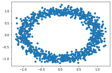
Above, we see a pretty clean circle. But what if the circle is in three dimensions?

def sample_noisy_sphere(n, **kw):
    """
    Sample n points uniformly at random from the k-sphere
    embedded in d dimensions.
    
    Add normal nosie with variance sigma
    
    Arguments:
        n - number of samples
    
    Optional arguments:
        r - radius of circle (default 1.0)
        k - dimension of sphere (default k = 1 == circle)
        sigma - noise variance (default 0.1)
        d - dimension of embedded space (default k+1)
    """
    r = kw.get('r', 1.0)
    k = kw.get('k', 1)
    sigma = kw.get('sigma', 0.1)
    d = kw.get('d', k+1)

    X = np.random.randn(n,k+1)
    X = r * X / np.linalg.norm(X, axis=1).reshape(n,-1) # project onto sphere
    
    Q, R = np.linalg.qr(np.random.randn(d, k+1))
    X = X @ Q.T # apply random rotation

    return X + sigma*np.random.randn(n,d)

(note: taking the Q factor of the QR decomposition of a random normal matrix is a good way to sample random subspaces)

m, n = 3,3
fig, ax = plt.subplots(m,n, figsize=(10,10))
for i in range(m):
    for j in range(n):
        X = sample_noisy_sphere(1000, d=5)

        ax[i,j].scatter(X[:,0], X[:,1])
        
plt.show(fig)

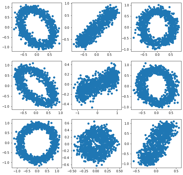
It isn’t always easy to see the circle in the scatter plot. This is because if we choose two dimensions arbitrarily, we don’t always align well with the rotated circle.

Plotly¶

Plotly is an open sourced graphing library which can help you create Javascript visualizations you can interact with in a web browser.

conda install plotly
conda install nbformat # you may need this

import plotly
import plotly.graph_objects as go

X = sample_noisy_sphere(1000, d=3)
fig = go.Figure(data=[go.Scatter3d(x=X[:,0], y=X[:,1], z=X[:,2],
                                   mode='markers', marker=dict(size=1))])
fig.show()

We’ll define a function for quick 3D scatter plots

def quick_scatter(X):
    fig = go.Figure(data=[go.Scatter3d(x=X[:,0], y=X[:,1], z=X[:,2],
                                   mode='markers',marker=dict(size=1))])
    fig.show()

Dimension Reduction¶

Dimension reduction is the process of taking a high-dimensional data set and embedding it in a lower dimension.

Often, data with many features is really generated by a process with only a handful of parameters. This typically means we can think of data being sampled from a low-dimensional (parameter) space, but embedded in a high-dimensional feature space (perhaps with some noise).

Dimension reduction algorithms seek to reverse this process - we want to go from the high dimensional feature space to a lower dimensional space where the data generating mechanism may be easier to reason about.

Principal Component Analysis (PCA)¶

The simplest way to reduce the dimension of real-valued data is through a linear projection.

X = sample_noisy_sphere(1000, d=100, sigma=0.1)
Q, R = np.linalg.qr(np.random.randn(X.shape[1], 3))
X2 = X @ Q

quick_scatter(X)

Clearly, a random projection isn’t necessarily the most useful. We want the best possible subspace to project onto. PCA defines the best $d$-dimensional subspace as the $d$-dimensional subspace with the largest variance in the data.

Recall that we can calculate the population variance using $$\hat{\Sigma} = \frac{1}{n}X^T X$$ Where we assume $X$ has zero mean (i.e $\tfrac{1}{n} 1^T X = 0$)

Let $v$ be a unit vector. The projection onto the subspace spanned by $v$ is calculated as $X v$. Note that if $X$ has zero-mean that $Xv$ will also have zero mean (prove it). The variance in this 1-dimensional subspace is then $$\sigma(v) = \frac{1}{n} (Xv)^T (Xv) = \frac{1}{n} v^T X^T X v$$

So the subspace with the largest variance is defined by the unit vector $v$ which maximizes $$v^T (\frac{1}{n} X^T X) v = v^T \hat{\Sigma} v$$

We can write this as the variational problem $$ \operatorname{maximze}_{v\in \mathbb{R}^n} v^T \hat{\Sigma} v\\ \text{subject to } \|v\|_2 = 1 $$

We recognize this as the problem of finding the largest magnitude eigenpair of $\hat{\Sigma}$, where $v$ is the eigenvector, and the eigenvalue of $v$ is $\sigma(v)$ (prove it).

If we want to project into a $k+1$ dimensional space, we then find $$ \operatorname{maximze}_{v\in \mathbb{R}^n} v^T \hat{\Sigma} v\\ \text{subject to } \|v\|_2 = 1, v^T V_k = 0 $$ where $V_k = [v_1,\dots,v_k]$ spans the optimal $k$-dimensional subspace.

This boils down to finding the largest $k+1$ dimensional eigenspace of $\hat{\Sigma}$.

The vectors $v_1,\dots, v_k$ are known as the principal components of $X$

def mean_center(X):
    mu = np.average(X, axis=0) # 1^T X / n
    return X - mu

def variance(X):
    n = X.shape[0]
    X = mean_center(X)
    return X.T @ X / n

def principal_vectors(X, k=3):
    Sigma = variance(X)
    lam, V = np.linalg.eigh(Sigma)
    return V[:,-k:] # eigenvalues in increasing order

def pca_projection(X, k=3):
    V = principal_vectors(X, k=k)
    return X @ V


X = sample_noisy_sphere(1000, d=100, sigma=0.1)
Xpca = pca_projection(X, k=3)

quick_scatter(Xpca)

PCA Via the SVD¶

In practice, you should not compute PCA by forming $X^T X$. Why? Because if $X$ is ill-conditioned, then $X^T X$ will be even more ill conditioned.

What you should do is use the SVD of $X$. If $X = U \Sigma V^T$ then $$X^T X = V \Sigma^T U^T U \Sigma V^T = V \Sigma^2 V^T$$ Clearly, the right-singular vectors $V$ are the eigenvectors of $X^T X$.

Exercises¶

Write a function to project a design matrix X onto its top k principal components using the SVD.
Modify your function to use ARPACK via scipy.sparse.linalg.svds
What is the condition number $\kappa(X^T X)$ expressed in terms of $\kappa(X)$? (Hint)
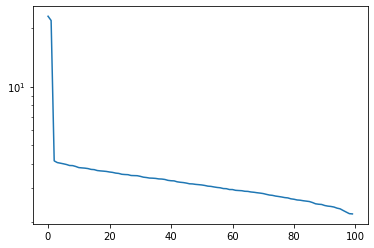
Plot the singular values of X generated above - how might you decide how many principal components to use?

# Your code here

X = sample_noisy_sphere(1000, d=100, sigma=0.1)
u, s, v = np.linalg.svd(X)
plt.semilogy(s)
plt.show()

Nonlinear Dimensionality Reduction¶

Often linear projections are not sufficient to visualize structure in data because an embedding into parameter space is not linear. There are a variety of techniques you can use for nonlinear dimensionality reduction.

These techniques often fall under the umbrella of “manifold learning” because we think if the parameter space describing the data as some manifold.

We’ll use Scikit-Learn’s manifold learning module to explore these algorithms.

conda install scikit-learn

Scikit-learn Syntax¶

Let’s go over how Scikit-Learn operates. We’ll use PCA as an example. See the documentation.

In general, Scikit-Learn provides objects that will perform some algorithm on data. In this case, we’ll use a PCA object.

from sklearn.decomposition import PCA

transformer = PCA(n_components=3)
type(transformer)

sklearn.decomposition._pca.PCA

There are two stages to using a dimension reduction technique.

First we “fit” an object (transformer above), to the data. Then we can transform X using the object.

X = sample_noisy_sphere(1000, d=100, sigma=0.01)
transformer.fit(X)
Xpca = transformer.transform(X)

quick_scatter(Xpca)

You can also use the combined fit_transform method

Xpca = transformer.fit_transform(X)
quick_scatter(Xpca)

Generating Nonlinear Data¶

Let’s make our data more interesting. First, we’ll generate some nested circles

def nested_spheres(*rs, **kw):
    """
    generate nested circles
    
    Arguments:
        r1, r2, r3,... radii of circles
        
    Optional arguments:
        n = number of samples for each circle (default 500)
        additional arguments will be passed to sample_noisy_sphere
    """
    ns = kw.pop('n', 500) # remove key from dict
    if type(ns) is int:
        ns = tuple(ns for r in rs)
      
    data = []
    for n, r in zip(ns, rs):
        data.append(sample_noisy_sphere(n, r=r, **kw))
        
    return np.concatenate(data, axis=0)

np.random.seed(1)
X = nested_spheres(1.0, 2.0, 3.0, d=3)
quick_scatter(X)

Y = X

We can also apply a non-linear function to the data

def f(x):
    y = [x[0]*x[1], x[0] - x[1], np.sin(x[1]), np.cos(x[1])]
    y.extend([x[i] for i in range(2, len(x))])
    return np.array(y)

Y = np.array([f(x) for x in X])
quick_scatter(Y)

We can see PCA is a bit convoluted:

Ypca = PCA().fit_transform(Y)
quick_scatter(Ypca)

Kernel PCA¶

Documentation

from sklearn.decomposition import KernelPCA
transformer = KernelPCA(n_components=3, kernel="rbf")
Ytrans = transformer.fit_transform(Y)
quick_scatter(Ytrans)

Isomap¶

import sklearn.manifold as manifold

transformer = manifold.Isomap(n_components=3)
Ytrans = transformer.fit_transform(Y)
quick_scatter(Ytrans)

Spectral Embedding¶

Spectral embeddings are computed from a graph obtained from the data. Typically, a weighted nearest neighbors graph.

transformer = manifold.SpectralEmbedding(n_components=3)
Ytrans = transformer.fit_transform(Y)
quick_scatter(Ytrans)

t-SNE¶

transformer = manifold.TSNE(n_components=3, init='pca', random_state=0)
Ytrans = transformer.fit_transform(Y)
quick_scatter(Ytrans)

Multidimensional Scaling¶

Let’s use a metric rather than the standard Euclidean metric

from scipy.spatial.distance import pdist, squareform # pairwise distances
D = squareform(pdist(Y, 'cityblock')) # L1 metric

transformer = manifold.MDS(n_components=3, dissimilarity="precomputed")
Ytrans = transformer.fit_transform(D)
quick_scatter(Ytrans)

Scientific Computing with Python

Dimension Reduction and Data Visualization

Contents