Integration & Quadrature
Contents
Integration & Quadrature
First, let’s recall a few definitions. An indefinite integral is an integral without bounds, and is defined up to a constant \begin{equation} \int x, dx = \frac{x^2}{2} + C \end{equation} A definite integral has bounds, which are sometimes symbolic \begin{equation} \int_0^y 1, dx = y \end{equation}
Symbolic Integration
sympy includes a variety of functionality for integration.
import sympy as sym
x, y = sym.symbols('x y')
You can compute indefinite integrals
sym.integrate(1, x)
sym.integrate(x**2 + x - 1)
sym.integrate(x*y, y)
If you want to compute definite integrals, you can pass in the bounds
sym.integrate(1, (x, 0, 2))
sym.integrate(sym.sin(x), (x, 0, sym.pi))
sym.integrate(x*y, (y, 0, 1))
sym.integrate(x, (x, 0, y))
SymPy also provides integral transforms such as the Fourier transform
k = sym.Symbol('k')
sym.fourier_transform(sym.exp(-x**2), x, k)
You can find more complete information in the sympy documentation
Numerical Integration (Quadrature)
Numerical integration is used to obtain definite integrals.
First, we should recall the definition of the Riemannian integral: \begin{equation} \int_a^b f(x), dx = \lim_{n\to \infty} \frac{b-a}{n}\sum_{i=1}^n f(x_i) (x_{i+1} - x_i) \end{equation} where the sequence \(\{x_i\}\) is built for each \(n\) so that \(x_{i+1} - x_{i} = (b-a)/n\). It is useful to think of how integrals compute area under a curve. In this case, we are (approximately) computing this area as the sum of rectangles with height \(f(x_i)\) and width \(x_{i+1}-x_i\). More generally, we can think of this as a weighted sum of function values \begin{equation} \sum_{i=1}^n f(x_i) w_i \end{equation} Which looks more like Lesbegue integration, where \(w_i\) is the measure assigned to the point \(x_i\).
In order to numerically integrate functions, we will take a finite sum of weighted function values, where the weights and function evaluation points are designed to give a good approximation to the integral. This is known as quadrature (instead of inegration).
Trapezoidal Rule
One of the simplest quadrature rules is trapezoid rule, which approximates an area under a curve by trapezoids defined by the four points \((x_i,0), (x_{i+1},0), (x_i, f(x_i)), (x_{i+1}, f(x_{i+1}))\). The area of this trapezoid is \begin{equation} \frac{1}{2}\bigg(f(x_{i+1}) + f(x_i)\bigg)(x_{i+1} - x_i) \end{equation} If we have \(a = x_0 \le x_1 \le ... \le x_{n} = b\) equally spaced, then the quadrature weights for \(x_i\) are \(w_i = (b-a)/n\) if \(i\notin \{0,n\}\), and \(w_i= (b-a)/(2n)\) if \(i \in \{0,n\}\)
You can use trapezoid rule in scipy using scipy.integrate.trapz
import numpy as np
from scipy.integrate import trapz

x = np.linspace(0,1,100)
y = x**2
trapz(y, x) # actual answer is 1/3
0.33335033840084355
Other quadrature rules that you can use easily are Simpson’s rule (simps) and Romberg’s rule (romb)
from scipy.integrate import simps

simps(y,x) # again, answer is 1/3
0.333333505101692
Gaussian Quadrature
Gaussian quadrature computes points x_i and weights w_i to optimally integrate polynomials up to some fixed order. This is all wrapped up in fixed_quad or quadrature functions
from scipy.integrate import fixed_quad, quadrature

f = lambda x: x**10
fixed_quad integrates up to fixed polynomial order
1/11
0.09090909090909091
fixed_quad(f, 0, 1, n=11) # n is order of polynomial
(0.09090909090909102, None)
The return tuple is the computed result and None.
quadrature integrates up to a fixed tolerance
quadrature(f, 0, 1)
(0.09090909090909097, 1.1102230246251565e-16)
for ifunction in (fixed_quad, quadrature):
    print(ifunction(f, 0, 1)[0])
0.09090765936004021
0.09090909090909097
The return tuple is the computed result and the error, measured as the difference between the last two estimates.
General Quadrature
The function quad wraps a varitety of functionality. Basic use is just like above
from scipy.integrate import quad

f = lambda x: x**2

quad(f, 0, 1)
(0.33333333333333337, 3.700743415417189e-15)
Again, the function returns the computed result, and an estimate of the absolute error.
You can also compute integrals on unbounded domains
f = lambda x: np.exp(-x**2)

quad(f, 0, np.inf)
(0.8862269254527579, 7.101318390472462e-09)
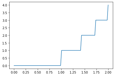
Functions with Discontinuities
Discontinuities can cause problems with any sort of quadrature scheme that assumes functions are continuous. You can specify problematics points with points
import matplotlib.pyplot as plt

f = lambda x : np.floor(x**2)

x = np.linspace(0,2,100)
plt.plot(x, f(x))
plt.show()
quad(f, 0, 2)
(1.8537356322944702, 9.277312917888025e-09)
quad(f, 0, 2, points=np.sqrt(np.arange(5)))
(1.8537356300580277, 2.0580599780584437e-14)
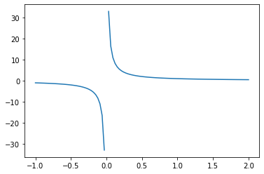
Functions with Singularities
Depending on the type of singularity, you can pass in different arguments into the weight and wvar parameters of quad. See the documentation for details.
For example, let’s say we want to compute
\begin{equation} \int_{-1}^2 \frac{1}{x},dx \end{equation}
f = lambda x : 1 / x

x = np.linspace(-1,2,100)
plt.plot(x, f(x))
plt.show()
<ipython-input-22-74bd56e45931>:1: RuntimeWarning: divide by zero encountered in true_divide
  f = lambda x : 1 / x
There is an odd symmetry in the interval \([-1,1]\), so we can calculate
\begin{equation} \int_{-1}^2 \frac{1}{x},dx = \int_1^2 \frac{1}{x},dx = \log(2) - \log(1) = \log(2) \end{equation}
The 'cauchy' weight will calculate the integral of \(\frac{f(x)}{x - {\tt wvar}}\) (i.e. we will weight the fuction \(f\) by the Cauchy distribution \(\frac{1}{x - {\tt wvar}}\)).
So we can use weight='cauchy' with wvar=0 on the function f(x) = 1 to compute our integral.
quad(lambda x : 1, -1, 2, weight='cauchy', wvar=0) # mulitply function by 1/x and do integration
(0.6931471805599452, 0.0)
np.log(2)
0.6931471805599453
Multivariate Integration
You can integrate over functions of multiple variables using
nquad integrates over a hyper cube defined by ranges in the second argument. dblquad and tplquad can allow you to integrate over more complicated domains.
from scipy.integrate import nquad

f = lambda x, y, z : np.exp( -x**2 - y**2 - z**2)

nquad(f, ((-3,3), (-3,3), (-3,3)))
(5.56795898358481, 1.4605401208842099e-08)
Monte Carlo Integration
Monte Carlo integration is a method which computes integrals by taking a sum over random samples.
\begin{equation} \int_{a}^b f(x) = \mathbb{E}_{U(a,b)} [f] \end{equation}
Where \(U(a,b)\) is the uniform distribution over the interval \([a,b]\). We can estimate this expected value by drawing samples from the distribution, and computing
\begin{equation} \mathbb{E}{U(a,b)} [f] \approx \frac{1}{N} \sum{i=1}^N f(x_i), x_i \sim U(a,b) \end{equation}
Or, more generally, we might define an integral over a probability measure \(\mu\)
\begin{equation} \int f(x), d\mu(x) = \mathbb{E}{\mu} [f] = \frac{1}{N} \sum{i=1}^N f(x_i), x_i \sim \mu(x) \end{equation}
The expected error can be derived from the law of large numbers, and is typically \(\frac{1}{\sqrt{N}}\). In high dimensions, this is typically the most effictive way to integrate functions, as quadrature requires a number of samples that is exponential in terms of the dimension.
Example
The classic example of Monte Carlo integration is computing \(\pi\) using random samples. Recall the area of the unit circle is \(\pi\), and the area of the square \([-1,1]^2\) is \(4\). We sample points uniformly from this square, and compute how many fall in the unit circle - the expected ratio of points inside the circle to the total number of points is \(\pi/4\).
def compute_pi_mc(n=1000):
    x = np.random.rand(n,2)*2 - 1 # sampled in [-1,1] x [-1,1]
    r = np.linalg.norm(x, axis=1) # computes radius of each point
    return 4 * np.sum(r <= 1.) / n
%time compute_pi_mc(10_000_000)
CPU times: user 390 ms, sys: 41.9 ms, total: 432 ms
Wall time: 433 ms
3.1413256
We can use numba to parallelize this
from numba import njit

@njit
def compute_pi_mc_numba(n=1000):
    x = np.random.rand(n,2)*2 - 1
    ct = 0
    for i in range(n):
        ct += x[i,0]**2 + x[i,1]**2 < 1
    return 4 * ct / n
%time compute_pi_mc_numba(10_000_000)
CPU times: user 749 ms, sys: 112 ms, total: 861 ms
Wall time: 880 ms
3.1416048
from numba import njit, prange

@njit(parallel=True)
def compute_pi_mc_numba_parallel(n=1000):
    x = np.random.rand(n,2)*2 - 1
    ct = 0
    for i in prange(n):
        ct += x[i,0]**2 + x[i,1]**2 < 1
    return 4 * ct / n
%time compute_pi_mc_numba_parallel(10_000_000)
CPU times: user 1.21 s, sys: 190 ms, total: 1.4 s
Wall time: 966 ms
3.1408412
if we look at the wall time, we see this runs faster than any of the other options