Sparse Linear Algebra¶

So far, we have seen how sparse matrices and linear operators can be used to speed up basic matrix-vector and matrix-matrix operations, and decrease the memory footprint of the representation of a linear map.

Just as there are special data types for sparse and structured matrices, there are specialized linear algebra routines which allow you to take advantage of sparsity and fast matrix-vector products.

Routines for sparse linear algebra are found in scipy.sparse.linalg, which we’ll import as sla

%pylab inline
import scipy.sparse as sparse
import scipy.sparse.linalg as sla

Populating the interactive namespace from numpy and matplotlib

Sparse Direct Methods¶

This typically refers to producing a factorization of a sparse matrix for use in solving linear systems.

The thing to keep in mind is that many factorizations will generally be dense, even if the original matrix is sparse. E.g. eigenvalue decompositions, QR decomposition, SVD, etc. This means that if we compute a factorization, we are going to lose all the advantages we had from sparsity.

What we really want is a factorization where if A is sparse, the terms in the factorization are also sparse. The factorization where this is easiest to achieve is the LU decomposition. In general, the L and U terms will be more dense than A, and sometimes much more dense. However, we can seek a permuted version of the matrix A which will minimize the amount of “fill-in” which occurs. This is often done using “nested disection” algorithm, which is outside the scope of this course. If you ever need to do this explicitly, the METIS package is commonly used.

We’ll just use the function sla.splu (SParse LU) at a high level, which produces a factorization object that can be used to solve linear systems.

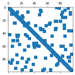
n = 100
A = sparse.random(n, n, 0.01) + sparse.eye(n)
plt.spy(A)
plt.show()

A = A.tocsc() # need to convert to CSC form first
LU = sla.splu(A)
LU

<SuperLU at 0x7fe016b4ea50>

The resulting object stores the factors necessary to compute A = PLUQ (P permutes rows, and Q permutes columns). It is computed using the SuperLU library. Typically, you will just use the solve method on this object.

x = np.random.randn(n)
b = A @ x

x2 = LU.solve(b)
print(np.linalg.norm(x2 - x))

7.892057678545134e-16

you can also use the sla.spsolve function, which wraps this factorization.

x2 = sla.spsolve(A, b)
print(np.linalg.norm(x2 - x))

7.892057678545134e-16

Sparse Iterative Methods¶

Sparse iterative methods are another class of methods you can use for solving linear systems built on Krylov subspaces. They only require matrix-vector products, and are ideally used with sparse matrices and fast linear operators. You can typically learn the theory behind these methods in a numerical linear algebra course - we’ll just talk about how to use them.

All these methods are meant to solve linear systems: find x so that A @ x = b, or least squares problems minimizing norm(A @ x - b)

You can find a list of options in the documentation for scipy.sparse.linalg. Here are some common options:

Conjugate Gradient: sla.cg for A SPD
MINRES: sla.minres for A symmetric
GMRES: sla.gmres for general square A
LSQR: sla.lsqr for solving least squares problems

For example, we can use gmres with the same matrix we used for splu:

x2, exit = sla.gmres(A, b, tol=1e-8) # exit code: 0 if successful
print(np.linalg.norm(x2 - x))

1.8840644705608314e-09

import time
x2 = np.empty_like(x)

t0 = time.time()
x2, exit = sla.gmres(A, b)
t1 = time.time()
print("GMRES in {} sec.".format(t1 - t0))

t0 = time.time()
x2 = sla.spsolve(A, b)
t1 = time.time()
print("spsolve in {} sec.".format(t1 - t0))

GMRES in 0.0008156299591064453 sec.
spsolve in 0.0004031658172607422 sec.

Sparse Direct vs. Iterative Methods¶

There are a couple of trade offs to consider when deciding whether to use sparse direct or iterative algorithms.

Are you going to be solving many linear systems with the same matrix A? If so, you can produce a single factorization object using splu, and use it to solve many right-hand sides. Sparse direct probably makes more sense.
Are you solving a single linear system? If so, then a single call to an iterative method probably makes mores sense.
Are you using a fast linear operator that could be expressed as a dense matrix (e.g. sparse plus low-rank)? Alternatively, would the sparse LU decomposition turn dense because of fill-in? If so, then iterative methods probably make more sense.
Do you have a really good preconditioner (see below)? Then iterative methods probably make more sense.

Preconditioning¶

The speed/effectiveness of iterative methods is often dependent on the existence of a good preconditioner. A preconditioner M for a matrix A is an “approximate inverse” i.e. M @ A is close to the identity. Note if we had an exact inverse, we’ve solved our problem already. What we want is to have a matrix M which is fast to apply (i.e. also sparse like A), which generally isn’t possible with an exact inverse.

Finding a good preconditioner is a huge field of research, and can be very domain-dependent. A general-purpose method to obtain a preconditioner is to use an Incomplete LU decomposition (this is an LU factorization that stops when the fill-in gets too large). You can obtain one using sla.spilu.

ILUfact = sla.spilu(A)
ILUfact

<SuperLU at 0x7fe016b1d270>

x = np.random.randn(n)
b = A @ x

x2 = LU.solve(b)
print(np.linalg.norm(x - x2))
x3 = ILUfact.solve(b)
print(np.linalg.norm(x - x3))

1.1781876100516644e-15
0.00020301844173399326

You can construct a preconditioner using a LinearOperator around the ILU object’s solve method

M = sla.LinearOperator(
    shape = A.shape,
    matvec = lambda b: ILUfact.solve(b)
)

x2, exit = sla.gmres(A, b, M=M) # exit code: 0 if successful
print(np.linalg.norm(x2 - x))

2.4705799953272913e-15

t0 = time.time()
x2, exit = sla.gmres(A, b)
t1 = time.time()
print("GMRES in {:.3e} sec.".format(t1 - t0))
print(np.linalg.norm(x2 - x))

t0 = time.time()
x2, exit = sla.gmres(A, b, M=M)
t1 = time.time()
print("preconditioned GMRES in {:.3e} sec.".format(t1 - t0))
print(np.linalg.norm(x2 - x))

GMRES in 1.076e-03 sec.
0.00013444484628655706
preconditioned GMRES in 1.052e-03 sec.
2.4705799953272913e-15

We get a higher-precision answer in about the same amount of time.

Eigenvalues and Eigenvectors¶

Computing a full eigenvalue decomposition of a sparse matrix or fast linear operator doesn’t typically make sense (see the the discussion for sparse direct methods). However, there are a lot of situations in which we want to compute the eigenvalue-eigenvector pairs for a handful of the largest (or smallest) eigenvalues.

scipy.sparse.linalg wraps ARPACK (ARnoldi PACKage), which uses Krylov subspace techniques (like the iterative methods) to compute eigenvalues/eigenvectors using matrix-vector multiplications. The relevant methods are sla.eigs (for general square matrices) and sla.eigsh (for symmetric/Hermitian matrices). There is also a sla.svds function for the SVD.

Let’s look at an example for a linear operator which acts as the matrix of all ones.

# works on square matrices
Afun = lambda X : np.sum(X, axis=0).reshape(1,-1).repeat(X.shape[0], axis=0)

m =10 # linear operator of size 10

A = sla.LinearOperator(
    shape   = (m,m),
    matvec  = Afun,
    rmatvec = Afun,
    matmat  = Afun,
    rmatmat = Afun,
    dtype=np.float   
)

This operator is Hermitian, so we’ll use eigsh. By default, eigsh will compute the largest magnitude eigenvalues. You can change which eigenvalues you’re looking for using the which keyword argument, and the number of eigenvalues using the k argument. See the documentation for details.

Lam, V = sla.eigsh(A, which='LM', k=4)

Lam

array([-5.86174617e-18, -3.50871500e-32,  1.78221859e-15,  1.00000000e+01])

we see there is one eigenvalue with a numerically non-zero value (10). Let’s take a look at the eigenvector

V[:,-1]

array([-0.31622777, -0.31622777, -0.31622777, -0.31622777, -0.31622777,
       -0.31622777, -0.31622777, -0.31622777, -0.31622777, -0.31622777])

this is the vector with constant entries. This agrees with our understanding of the operator A, which can be expressed as the symmetric rank-1 outer product of the vector with 1s in every entry.

Randomized Linear Algebra¶

In the past decade or two, randomized linear algebra has matured as a topic with lots of practical applications. To read about the theory, see the 2009 paper by Halko, Martinsson, and Tropp: Link.

SciPy does not (currently) have built-in functions for randomized linear algebra functionality (some languages like Julia do). Fortunately, these algorithms are very easy to implement without worrying too much about the theory.

For simplicity, we’ll assume that A is symmetric with distinct eigenvectors, so we can limit the discussion to eigenvectors. A rank-k approximation of A is an approximation by a rank-k outer product. We can analyitically obtain the optimal rank-k approximation by computing a full eigenvalue decomposition of A and set all the eigenvalues outside the largest k (in magnitude) to 0. Again, we don’t want to actually compute the full eigenvalue decomposition, so we want an algorithm that does this in some provable way.

The basic idea is to get an approximation of the range of an operator A by applying it to a bunch of random vectors. That is, we compute A @ X, where X is a matrix with random entries (we think of every column as a random vector). One way to think about the action of A is that it “rotates” these random vectors preferentially in the direction of the top eigenvectors, so if we look at the most important subspace of the span of the image A @ X (as measured by the svd), we get a good approximation of the most important eigenspace.

Randomized algorithms have probabilistic gurarantees. The statement is roughly that if entries of X are iid sub-Gaussian random variables (you can replace “sub-Gaussian” with Gaussian), and if we use k+p random vectors (p is a small constant), we can get close to the top-k dimensional eigenspace with high probability. In this case, close depends on something called the spectral gap, and with high probability means that in order to not be close to the desired subspace you would likely need to keep running computations with different random numbers for millions or billions of years before you would observe the algorithm fail.

Let’s see how this works in practice:

import scipy.linalg as la

def random_span_k_svd(A, k, p=10, power=0):
    """
    Compute subspace whose span is close to contaning the top-k eigenspace of A
    
    p = number of dimensions to pad
    power : number of times to run a power iteration on the subspace
    """
    m, n = A.shape
        
    X = np.random.randn(n, k+p)
    Y = A @ X
    
    U, s, Vt = la.svd(Y, full_matrices=False)
    
    for i in range(power):
        Y = A @ U
        U, s, Vt = la.svd(Y, full_matrices=False)
    
    
    return U

Here’s a version that uses orgqr from LAPACK

from scipy.linalg import lapack

def random_span_k(A, k, p=10, power=0):
    """
    Compute subspace whose span is close to contaning the top-k eigenspace of A
    
    p = number of dimensions to pad
    power : number of times to run a power iteration on the subspace
    """
    m, n = A.shape
        
    X = np.random.randn(n, k+p)
    Y = A @ X
    
    m, n = Y.shape
    lwork = max(3*n, 1)
    qr, tau, work, info = lapack.dgeqrf(Y, lwork, 1) # overwrite A = True
    Y, work, info = lapack.dorgqr(qr, tau, lwork, 1) # overwrite qr = True
    
    for i in range(power):
        Y = A @ Y
        qr, tau, work, info = lapack.dgeqrf(Y, lwork, 1) # overwrite A = True
        Y, work, info = lapack.dorgqr(qr, tau, lwork, 1) # overwrite qr = True
    
    
    return Y

Let’s test this on a diagonal matrix with entries 0 to n-1 along the main diagonal. In this case, the eigenvalues are integers, and the eigenvectors are the standard basis vectors.

n = 100
D = sparse.dia_matrix((np.arange(n), [0]), shape=(n,n))
D

<100x100 sparse matrix of type '<class 'numpy.int64'>'
	with 100 stored elements (1 diagonals) in DIAgonal format>

Let’s compare the two versions

k = 5

%timeit U = random_span_k_svd(D, k)

398 µs ± 4.57 µs per loop (mean ± std. dev. of 7 runs, 1000 loops each)

%timeit U = random_span_k(D, k)

289 µs ± 12.3 µs per loop (mean ± std. dev. of 7 runs, 1000 loops each)

k = 5
U = random_span_k(D, k)

lam, V = la.eigh(D.todense())
V_true = V[:,-k:]
V_true[-k:,:] # should see identity

array([[1., 0., 0., 0., 0.],
       [0., 1., 0., 0., 0.],
       [0., 0., 1., 0., 0.],
       [0., 0., 0., 1., 0.],
       [0., 0., 0., 0., 1.]])

Let’s take a look at how well U captures each eigenvector. The distance from this subspace from the ith eigenvector is norm(V[:,i].T*U). Because the eigenvectors are canonical basis vectors, this is just the norm of the ith row of U

Ui_norms = []
for i in range(n):
    Ui_norms.append(np.linalg.norm(U[i]))
#     print("{:02d} : {}".format(i, np.linalg.norm(U[i])))

plt.plot(Ui_norms)
plt.xlabel('eigenvector')
plt.ylabel('weight')
plt.show()

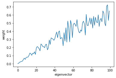
As we see, U is closer to the larger eigenvectors, rather than the smaller eigenvectors.

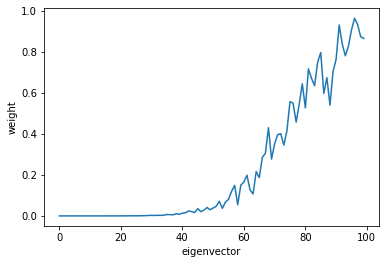
We can improve this estimate by running a couple of power iterations on the subspace (the power keyword defined above):

U = random_span_k(D, k, power=5)
Ui_norms = []
for i in range(n):
    Ui_norms.append(np.linalg.norm(U[i]))
    
#     print("{:02d} : {}".format(i, np.linalg.norm(U[i])))

plt.plot(Ui_norms)
plt.xlabel('eigenvector')
plt.ylabel('weight')
plt.show()

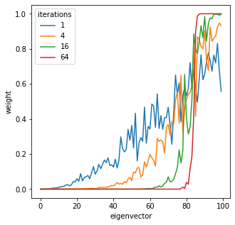
powers = [1, 4, 16, 64]

fig, ax = plt.subplots(figsize=(5,5))

for pi, power in enumerate(powers):
    U = random_span_k(D, k, power=power)
    Ui_norms = []
    for i in range(n):
        Ui_norms.append(np.linalg.norm(U[i]))

    #     print("{:02d} : {}".format(i, np.linalg.norm(U[i])))

    ax.plot(Ui_norms, label="{}".format(power))
    
ax.set_xlabel('eigenvector')
ax.set_ylabel('weight')

plt.legend(title='iterations')
plt.show()

U.shape

(100, 15)

Exercises¶

Download a couple of test matrices from the UFlorida Sparse Matrix collection Link For, example, use mnist_test_norm_10NN Link which would probably be too large to store on your computer as a dense matrix.

For each square matrix:

Solve a random linear system using splu
Solve a random linear system using either minres or gmres (which one should you use?)
Compute the largest magnitude eigenvector using eigs or eigsh (which one should you use?)

Find a non-square matrix and

Solve a random least squares problem using lsqr
Compute the largest singular vectors using svds

## Your code here

fname = '1138_bus.mtx'
data = np.genfromtxt(fname, comments='%') # skip any rows that begin with `%`
data.shape

m, n = int(data[0,0]), int(data[0,1])
data = data[1:]

rows = data[:,0] - 1
cols = data[:,1] - 1
vals = data[:,2]
A = sparse.coo_matrix((vals, (rows, cols)), shape=(m,n))
A = A.tocsc()
A

<1138x1138 sparse matrix of type '<class 'numpy.float64'>'
	with 2596 stored elements in Compressed Sparse Column format>

Direct method

LU = sla.splu(A)

np.random.seed(0)
x = np.random.randn(n)
b = A @ x

x2 = LU.solve(b)
print(np.linalg.norm(x2 - x))

3.729624510424685e-15

Iterative method. matrix is not symmetric, so use GMRES

x3, exit_status = sla.gmres(A, b)
print(np.linalg.norm(x3 - x))

1.1062499070369447

GMRES is very imprecise here, try preconditioning

ILUfact = sla.spilu(A)

M = sla.LinearOperator(
    shape = A.shape,
    matvec = lambda b: ILUfact.solve(b)
)

x3, exit_status = sla.gmres(A, b, M=M)
print(np.linalg.norm(x3 - x))

4.777111230904957e-07

Scientific Computing with Python

Sparse Linear Algebra

Contents