.ipynb .pdf

repository open issue

Binder Colab

Contents

SciKit Learn

Scikit-learn is a library that allows you to do machine learning, that is, make predictions from data, in Python. There are four basic tasks:

1. Regression: predict a number from data points, given data points and corresponding numbers

2. Classification: predict a category from datapoints, given data points and corresponding numbers

3. Clustering: predict a category from data points, given only data points

4. Dimensionality reduction: make data points lower-dimensional so that we can visualize the data

Here is a flowchart from the scikit learn documentation of when to use each technique.

You may need to install scikit learn

(pycourse) conda install scikit-learn

import pandas as pd
import numpy as np
import matplotlib.pyplot as plt
import sklearn # scikit-learn

Data Sets

A good place to look for example data sets to use in machine learning tasks is the UCI Machine Learning Repository

This repository (currently) contains 559 data sets, including information on where they came from and how to use them.

On this page we’ll use the Iris and Abalone data sets.

The Iris data set consists of measurements of three species of Iris (a flower). The Abalone data set consists of meaurements of abalone, a type of edible marine snail.

You can download the data by going to the data folder for each data set (here is the one for Iris). You will see a file with the extension *.data which is a csv file containing the data. This file does not have a header - you need to look at the attribute information on the data set home page to get the attribute names.

Scikit learn also has a few built-in data sets for easy loading:

from sklearn import datasets

Some of these can also be found in the UCI repository.

Regression

Abalone are a type of edible marine snail, and they have internal rings that correspond to their age (like trees). In the following, we will the dataset of abalone measurements. It has the following fields:

Sex / nominal / -- / M, F, and I (infant) 
Length / continuous / mm / Longest shell measurement 
Diameter	/ continuous / mm / perpendicular to length 
Height / continuous / mm / with meat in shell 
Whole weight / continuous / grams / whole abalone 
Shucked weight / continuous	/ grams / weight of meat 
Viscera weight / continuous / grams / gut weight (after bleeding) 
Shell weight / continuous / grams / after being dried 
Rings / integer / -- / +1.5 gives the age in years 

Suppose we are interested in predicting the age of the abalone given their measurements. This is an example of a regression problem.

df = pd.read_csv('http://archive.ics.uci.edu/ml/machine-learning-databases/abalone/abalone.data',
                   header=None, names=['sex', 'length', 'diameter', 'height', 'weight', 'shucked_weight',
                                       'viscera_weight', 'shell_weight', 'rings'])
df

	sex	length	diameter	height	weight	shucked_weight	viscera_weight	shell_weight	rings
0	M	0.455	0.365	0.095	0.5140	0.2245	0.1010	0.1500	15
1	M	0.350	0.265	0.090	0.2255	0.0995	0.0485	0.0700	7
2	F	0.530	0.420	0.135	0.6770	0.2565	0.1415	0.2100	9
3	M	0.440	0.365	0.125	0.5160	0.2155	0.1140	0.1550	10
4	I	0.330	0.255	0.080	0.2050	0.0895	0.0395	0.0550	7
...	...	...	...	...	...	...	...	...	...
4172	F	0.565	0.450	0.165	0.8870	0.3700	0.2390	0.2490	11
4173	M	0.590	0.440	0.135	0.9660	0.4390	0.2145	0.2605	10
4174	M	0.600	0.475	0.205	1.1760	0.5255	0.2875	0.3080	9
4175	F	0.625	0.485	0.150	1.0945	0.5310	0.2610	0.2960	10
4176	M	0.710	0.555	0.195	1.9485	0.9455	0.3765	0.4950	12

4177 rows × 9 columns

df.describe()

	length	diameter	height	weight	shucked_weight	viscera_weight	shell_weight	rings
count	4177.000000	4177.000000	4177.000000	4177.000000	4177.000000	4177.000000	4177.000000	4177.000000
mean	0.523992	0.407881	0.139516	0.828742	0.359367	0.180594	0.238831	9.933684
std	0.120093	0.099240	0.041827	0.490389	0.221963	0.109614	0.139203	3.224169
min	0.075000	0.055000	0.000000	0.002000	0.001000	0.000500	0.001500	1.000000
25%	0.450000	0.350000	0.115000	0.441500	0.186000	0.093500	0.130000	8.000000
50%	0.545000	0.425000	0.140000	0.799500	0.336000	0.171000	0.234000	9.000000
75%	0.615000	0.480000	0.165000	1.153000	0.502000	0.253000	0.329000	11.000000
max	0.815000	0.650000	1.130000	2.825500	1.488000	0.760000	1.005000	29.000000

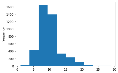
df['rings'].plot.hist()
plt.show()

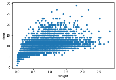
df.plot.scatter('weight', 'rings')
plt.show()

X = df[['weight']].to_numpy()
y = df['rings'].to_numpy()

X, y

(array([[0.514 ],
        [0.2255],
        [0.677 ],
        ...,
        [1.176 ],
        [1.0945],
        [1.9485]]),
 array([15,  7,  9, ...,  9, 10, 12]))

from sklearn import linear_model
model = linear_model.LinearRegression()
model.fit(X, y)
print("slope: {}, intercept: {}".format(model.coef_, model.intercept_))
print("score: {}".format(model.score(X, y)))

slope: [3.55290921], intercept: 6.989238807755703
score: 0.29202100292591804

# predict number of rings based on new weight observations
model.predict(np.array([[1.5], [2.2]]))

array([12.31860263, 14.80563908])

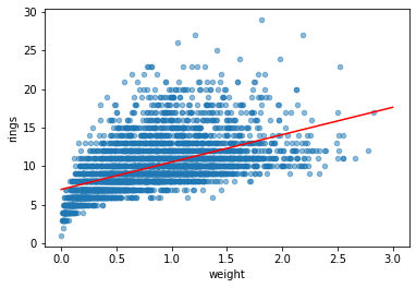
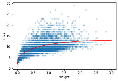
df.plot.scatter('weight', 'rings', alpha=0.5)

weight = np.linspace(0, 3, 10).reshape(-1, 1)
plt.plot(weight, model.predict(weight), 'r')

[<matplotlib.lines.Line2D at 0x7fba609c4190>]

# create a new feature: sqrt(weight)
df['root_weight'] = np.sqrt(df['weight'])

X = df[['weight','root_weight']].to_numpy()
y = df['rings'].to_numpy()
model = linear_model.LinearRegression()
model.fit(X, y)

LinearRegression()

weight = np.linspace(0, 3, 100).reshape(-1, 1)
root_weight = np.sqrt(weight)
features = np.hstack((weight,root_weight))

df.plot.scatter('weight', 'rings', alpha=0.2)
plt.plot(weight, model.predict(features), 'r')
plt.show()

model.coef_

array([-3.57798188, 12.36414363])

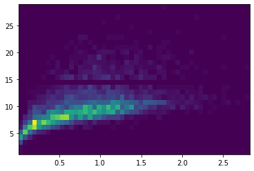
plt.hist2d(df['weight'], df['rings'],bins=(50,30));

from sklearn import linear_model
model = linear_model.LinearRegression()
model.fit(X, y)
print("slope: {}, intercept: {}".format(model.coef_, model.intercept_))
print("score: {}".format(model.score(X, y)))

slope: [-3.57798188 12.36414363], intercept: 2.226216110976191
score: 0.34587406410396215

# from sklearn import linear_model
model = linear_model.ElasticNet()
model.fit(X, y)
print("slope: {}, intercept: {}".format(model.coef_, model.intercept_))
print("score: {}".format(model.score(X, y)))

slope: [0.47838006 0.        ], intercept: 9.537230735081708
score: 0.07334400778940353

Classification

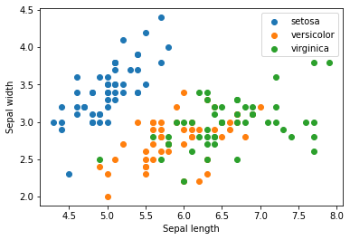
Another example of a machine learning problem is classification. Here we will use a dataset of flower measurements from three different flower species of Iris (Iris setosa, Iris virginica, and Iris versicolor). We aim to predict the species of the flower. Because the species is not a numerical output, it is not a regression problem, but a classification problem.

from sklearn import datasets
iris = datasets.load_iris()
print(iris.DESCR)

.. _iris_dataset:

Iris plants dataset
--------------------

**Data Set Characteristics:**

    :Number of Instances: 150 (50 in each of three classes)
    :Number of Attributes: 4 numeric, predictive attributes and the class
    :Attribute Information:
        - sepal length in cm
        - sepal width in cm
        - petal length in cm
        - petal width in cm
        - class:
                - Iris-Setosa
                - Iris-Versicolour
                - Iris-Virginica
                
    :Summary Statistics:

    ============== ==== ==== ======= ===== ====================
                    Min  Max   Mean    SD   Class Correlation
    ============== ==== ==== ======= ===== ====================
    sepal length:   4.3  7.9   5.84   0.83    0.7826
    sepal width:    2.0  4.4   3.05   0.43   -0.4194
    petal length:   1.0  6.9   3.76   1.76    0.9490  (high!)
    petal width:    0.1  2.5   1.20   0.76    0.9565  (high!)
    ============== ==== ==== ======= ===== ====================

    :Missing Attribute Values: None
    :Class Distribution: 33.3% for each of 3 classes.
    :Creator: R.A. Fisher
    :Donor: Michael Marshall (MARSHALL%PLU@io.arc.nasa.gov)
    :Date: July, 1988

The famous Iris database, first used by Sir R.A. Fisher. The dataset is taken
from Fisher's paper. Note that it's the same as in R, but not as in the UCI
Machine Learning Repository, which has two wrong data points.

This is perhaps the best known database to be found in the
pattern recognition literature.  Fisher's paper is a classic in the field and
is referenced frequently to this day.  (See Duda & Hart, for example.)  The
data set contains 3 classes of 50 instances each, where each class refers to a
type of iris plant.  One class is linearly separable from the other 2; the
latter are NOT linearly separable from each other.

.. topic:: References

   - Fisher, R.A. "The use of multiple measurements in taxonomic problems"
     Annual Eugenics, 7, Part II, 179-188 (1936); also in "Contributions to
     Mathematical Statistics" (John Wiley, NY, 1950).
   - Duda, R.O., & Hart, P.E. (1973) Pattern Classification and Scene Analysis.
     (Q327.D83) John Wiley & Sons.  ISBN 0-471-22361-1.  See page 218.
   - Dasarathy, B.V. (1980) "Nosing Around the Neighborhood: A New System
     Structure and Classification Rule for Recognition in Partially Exposed
     Environments".  IEEE Transactions on Pattern Analysis and Machine
     Intelligence, Vol. PAMI-2, No. 1, 67-71.
   - Gates, G.W. (1972) "The Reduced Nearest Neighbor Rule".  IEEE Transactions
     on Information Theory, May 1972, 431-433.
   - See also: 1988 MLC Proceedings, 54-64.  Cheeseman et al"s AUTOCLASS II
     conceptual clustering system finds 3 classes in the data.
   - Many, many more ...

X = iris.data[:, :2]
y = iris.target_names[iris.target]

for name in iris.target_names:
    plt.scatter(X[y == name, 0], X[y == name, 1], label=name)
plt.xlabel('Sepal length')
plt.ylabel('Sepal width')
plt.legend();

from sklearn.model_selection import train_test_split
X_train, X_test, y_train, y_test = train_test_split(X, y, test_size=0.2, random_state=1)
print(X_train.shape, y_train.shape)
print(X_test.shape, y_test.shape)

(120, 2) (120,)
(30, 2) (30,)

from sklearn.neighbors import KNeighborsClassifier
model = KNeighborsClassifier()
model.fit(X_train, y_train)

KNeighborsClassifier()

X_test

array([[5.8, 4. ],
       [5.1, 2.5],
       [6.6, 3. ],
       [5.4, 3.9],
       [7.9, 3.8],
       [6.3, 3.3],
       [6.9, 3.1],
       [5.1, 3.8],
       [4.7, 3.2],
       [6.9, 3.2],
       [5.6, 2.7],
       [5.4, 3.9],
       [7.1, 3. ],
       [6.4, 3.2],
       [6. , 2.9],
       [4.4, 3.2],
       [5.8, 2.6],
       [5.6, 3. ],
       [5.4, 3.4],
       [5. , 3.2],
       [5.5, 2.6],
       [5.4, 3. ],
       [6.7, 3. ],
       [5. , 3.5],
       [7.2, 3.2],
       [5.7, 2.8],
       [5.5, 4.2],
       [5.1, 3.8],
       [6.1, 2.8],
       [6.3, 2.5]])

model.predict(X_test)

array(['setosa', 'versicolor', 'virginica', 'setosa', 'virginica',
       'virginica', 'virginica', 'setosa', 'setosa', 'virginica',
       'versicolor', 'setosa', 'virginica', 'virginica', 'versicolor',
       'setosa', 'versicolor', 'versicolor', 'setosa', 'setosa',
       'versicolor', 'versicolor', 'virginica', 'setosa', 'virginica',
       'versicolor', 'setosa', 'setosa', 'versicolor', 'virginica'],
      dtype='<U10')

Evaluating your model

np.mean(model.predict(X_test) == y_test)  # Accuracy

0.8666666666666667

import sklearn.metrics as metrics
metrics.accuracy_score(model.predict(X_test), y_test)

0.8666666666666667

print(metrics.classification_report(model.predict(X_test), y_test))

              precision    recall  f1-score   support

      setosa       1.00      1.00      1.00        11
  versicolor       0.69      1.00      0.82         9
   virginica       1.00      0.60      0.75        10

    accuracy                           0.87        30
   macro avg       0.90      0.87      0.86        30
weighted avg       0.91      0.87      0.86        30

# Cross validation
from sklearn.model_selection import cross_val_score
model = KNeighborsClassifier()
scores = cross_val_score(model, X, y, cv=5)
scores

array([0.7       , 0.76666667, 0.73333333, 0.86666667, 0.76666667])

print(f"Accuracy: {scores.mean()} (+/- {scores.std()})")

Accuracy: 0.7666666666666667 (+/- 0.05577733510227173)

Using the full data - before we just used the first 2 features.

X = iris.data
y = iris.target_names[iris.target]
X_train, X_test, y_train, y_test = train_test_split(X, y, test_size=0.2, random_state=0)
model = KNeighborsClassifier(5)
model.fit(X_train, y_train)
print(metrics.classification_report(model.predict(X_test), y_test))

              precision    recall  f1-score   support

      setosa       1.00      1.00      1.00        11
  versicolor       0.92      1.00      0.96        12
   virginica       1.00      0.86      0.92         7

    accuracy                           0.97        30
   macro avg       0.97      0.95      0.96        30
weighted avg       0.97      0.97      0.97        30

Exercise

Try to fit some of the models in the following cell to the same data. Compute the relevant statistics (e.g. accuracy, precision, recall). Look up the documentation for the classifier, and see if the classifier takes any parameters. How does changing the parameter affect the result?

from sklearn.neural_network import MLPClassifier
from sklearn.svm import SVC
from sklearn.gaussian_process import GaussianProcessClassifier
from sklearn.tree import DecisionTreeClassifier
from sklearn.ensemble import RandomForestClassifier, AdaBoostClassifier
from sklearn.naive_bayes import GaussianNB
from sklearn.discriminant_analysis import QuadraticDiscriminantAnalysis

models = [
    # MLP classifier doesn't converge without additional iterations and learning rate adjustments, so define those here.
    MLPClassifier(learning_rate='adaptive', max_iter=1000), 
    SVC(), 
    GaussianProcessClassifier(max_iter_predict=20), 
    GaussianProcessClassifier(max_iter_predict=200), # 10x the training iterations won't even improve model fit, sadly
    DecisionTreeClassifier(), 
    RandomForestClassifier(), 
    AdaBoostClassifier(), 
    AdaBoostClassifier(learning_rate=0.5), # Decreasing our learning rate for this classifier can yield slightly better fit
    GaussianNB(), 
    QuadraticDiscriminantAnalysis() # QDA classifier gives us our overall best fit (~98%)
]

def trainAndEvaluate(model):
    print(f"Evaluating {type(model).__name__}:")

    X = iris.data
    y = iris.target_names[iris.target]
    X_train, X_test, y_train, y_test = train_test_split(X, y, test_size=0.2, random_state=0)
    model.fit(X_train, y_train)
    
    scores = cross_val_score(model, X, y, cv=5)
    
    print(metrics.classification_report(model.predict(X_test), y_test))
    print(f"Accuracy: {scores.mean()} (+/- {scores.std()})")  
    print("\n====================================================")

for model in models:
    modelName = type(model).__name__
    trainAndEvaluate(model)

Evaluating MLPClassifier:

              precision    recall  f1-score   support

      setosa       1.00      1.00      1.00        11
  versicolor       1.00      1.00      1.00        13
   virginica       1.00      1.00      1.00         6

    accuracy                           1.00        30
   macro avg       1.00      1.00      1.00        30
weighted avg       1.00      1.00      1.00        30

Accuracy: 0.9800000000000001 (+/- 0.02666666666666666)

====================================================
Evaluating SVC:
              precision    recall  f1-score   support

      setosa       1.00      1.00      1.00        11
  versicolor       1.00      1.00      1.00        13
   virginica       1.00      1.00      1.00         6

    accuracy                           1.00        30
   macro avg       1.00      1.00      1.00        30
weighted avg       1.00      1.00      1.00        30

Accuracy: 0.9666666666666666 (+/- 0.02108185106778919)

====================================================
Evaluating GaussianProcessClassifier:
              precision    recall  f1-score   support

      setosa       1.00      1.00      1.00        11
  versicolor       1.00      1.00      1.00        13
   virginica       1.00      1.00      1.00         6

    accuracy                           1.00        30
   macro avg       1.00      1.00      1.00        30
weighted avg       1.00      1.00      1.00        30

Accuracy: 0.9733333333333334 (+/- 0.01333333333333333)

====================================================
Evaluating GaussianProcessClassifier:

              precision    recall  f1-score   support

      setosa       1.00      1.00      1.00        11
  versicolor       1.00      1.00      1.00        13
   virginica       1.00      1.00      1.00         6

    accuracy                           1.00        30
   macro avg       1.00      1.00      1.00        30
weighted avg       1.00      1.00      1.00        30

Accuracy: 0.9733333333333334 (+/- 0.01333333333333333)

====================================================
Evaluating DecisionTreeClassifier:
              precision    recall  f1-score   support

      setosa       1.00      1.00      1.00        11
  versicolor       1.00      1.00      1.00        13
   virginica       1.00      1.00      1.00         6

    accuracy                           1.00        30
   macro avg       1.00      1.00      1.00        30
weighted avg       1.00      1.00      1.00        30

Accuracy: 0.9600000000000002 (+/- 0.03265986323710903)

====================================================
Evaluating RandomForestClassifier:

              precision    recall  f1-score   support

      setosa       1.00      1.00      1.00        11
  versicolor       1.00      1.00      1.00        13
   virginica       1.00      1.00      1.00         6

    accuracy                           1.00        30
   macro avg       1.00      1.00      1.00        30
weighted avg       1.00      1.00      1.00        30

Accuracy: 0.9533333333333334 (+/- 0.03399346342395189)

====================================================
Evaluating AdaBoostClassifier:

              precision    recall  f1-score   support

      setosa       1.00      1.00      1.00        11
  versicolor       1.00      0.93      0.96        14
   virginica       0.83      1.00      0.91         5

    accuracy                           0.97        30
   macro avg       0.94      0.98      0.96        30
weighted avg       0.97      0.97      0.97        30

Accuracy: 0.9466666666666667 (+/- 0.03399346342395189)

====================================================
Evaluating AdaBoostClassifier:

              precision    recall  f1-score   support

      setosa       1.00      1.00      1.00        11
  versicolor       1.00      0.81      0.90        16
   virginica       0.50      1.00      0.67         3

    accuracy                           0.90        30
   macro avg       0.83      0.94      0.85        30
weighted avg       0.95      0.90      0.91        30

Accuracy: 0.9533333333333334 (+/- 0.03399346342395189)

====================================================
Evaluating GaussianNB:
              precision    recall  f1-score   support

      setosa       1.00      1.00      1.00        11
  versicolor       1.00      0.93      0.96        14
   virginica       0.83      1.00      0.91         5

    accuracy                           0.97        30
   macro avg       0.94      0.98      0.96        30
weighted avg       0.97      0.97      0.97        30

Accuracy: 0.9533333333333334 (+/- 0.02666666666666666)

====================================================
Evaluating QuadraticDiscriminantAnalysis:
              precision    recall  f1-score   support

      setosa       1.00      1.00      1.00        11
  versicolor       1.00      1.00      1.00        13
   virginica       1.00      1.00      1.00         6

    accuracy                           1.00        30
   macro avg       1.00      1.00      1.00        30
weighted avg       1.00      1.00      1.00        30

Accuracy: 0.9800000000000001 (+/- 0.02666666666666666)

====================================================

Clustering

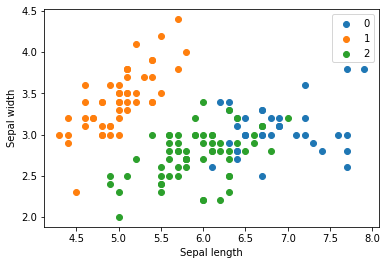
Clustering is useful if we don’t have a dataset labelled with the categories we want to predict, but we nevertheless expect there to be a certain number of categories. For example, suppose we have the previous dataset, but we are missing the labels. We can use a clustering algorithm like k-means to cluster the datapoints. Because we don’t have labels, clustering is what is called an unsupervised learning algorithm.

X = iris.data
for name in iris.target_names:
    plt.scatter(X[y == name, 0], X[y == name, 1], label=name)
plt.xlabel('Sepal length')
plt.ylabel('Sepal width')
plt.legend()
plt.show()

from sklearn.cluster import KMeans

model = KMeans(n_clusters=3, random_state=0)
model.fit(X)

KMeans(n_clusters=3, random_state=0)

model.labels_

array([1, 1, 1, 1, 1, 1, 1, 1, 1, 1, 1, 1, 1, 1, 1, 1, 1, 1, 1, 1, 1, 1,
       1, 1, 1, 1, 1, 1, 1, 1, 1, 1, 1, 1, 1, 1, 1, 1, 1, 1, 1, 1, 1, 1,
       1, 1, 1, 1, 1, 1, 2, 2, 0, 2, 2, 2, 2, 2, 2, 2, 2, 2, 2, 2, 2, 2,
       2, 2, 2, 2, 2, 2, 2, 2, 2, 2, 2, 0, 2, 2, 2, 2, 2, 2, 2, 2, 2, 2,
       2, 2, 2, 2, 2, 2, 2, 2, 2, 2, 2, 2, 0, 2, 0, 0, 0, 0, 2, 0, 0, 0,
       0, 0, 0, 2, 2, 0, 0, 0, 0, 2, 0, 2, 0, 2, 0, 0, 2, 2, 0, 0, 0, 0,
       0, 2, 0, 0, 0, 0, 2, 0, 0, 0, 2, 0, 0, 0, 2, 0, 0, 2], dtype=int32)

iris.target

array([0, 0, 0, 0, 0, 0, 0, 0, 0, 0, 0, 0, 0, 0, 0, 0, 0, 0, 0, 0, 0, 0,
       0, 0, 0, 0, 0, 0, 0, 0, 0, 0, 0, 0, 0, 0, 0, 0, 0, 0, 0, 0, 0, 0,
       0, 0, 0, 0, 0, 0, 1, 1, 1, 1, 1, 1, 1, 1, 1, 1, 1, 1, 1, 1, 1, 1,
       1, 1, 1, 1, 1, 1, 1, 1, 1, 1, 1, 1, 1, 1, 1, 1, 1, 1, 1, 1, 1, 1,
       1, 1, 1, 1, 1, 1, 1, 1, 1, 1, 1, 1, 2, 2, 2, 2, 2, 2, 2, 2, 2, 2,
       2, 2, 2, 2, 2, 2, 2, 2, 2, 2, 2, 2, 2, 2, 2, 2, 2, 2, 2, 2, 2, 2,
       2, 2, 2, 2, 2, 2, 2, 2, 2, 2, 2, 2, 2, 2, 2, 2, 2, 2])

for name in [0,1,2]:
    plt.scatter(X[model.labels_ == name, 0], X[model.labels_ == name, 1], label=name)
plt.xlabel('Sepal length')
plt.ylabel('Sepal width')
plt.legend()
plt.show()

X = iris.data
for name in iris.target_names:
    plt.scatter(X[y == name, 0], X[y == name, 1], label=name)
plt.xlabel('Sepal length')
plt.ylabel('Sepal width')
plt.legend()
plt.show()

Exercise

Load the breast cancer dataset.

• Try to cluster it into two clusters and check if the clusters match with the target class from the dataset, which specifies if its malignant or not. Here we are testing if we can we idenitify if its malignant or benign without even looking at the target class i.e. using unsupervised learning.

• Next, train a supervised classifier, a DecisionTreeClassifier, and see how much improvement we get

bc = datasets.load_breast_cancer()
print(bc.DESCR)

.. _breast_cancer_dataset:

Breast cancer wisconsin (diagnostic) dataset
--------------------------------------------

**Data Set Characteristics:**

    :Number of Instances: 569

    :Number of Attributes: 30 numeric, predictive attributes and the class

    :Attribute Information:
        - radius (mean of distances from center to points on the perimeter)
        - texture (standard deviation of gray-scale values)
        - perimeter
        - area
        - smoothness (local variation in radius lengths)
        - compactness (perimeter^2 / area - 1.0)
        - concavity (severity of concave portions of the contour)
        - concave points (number of concave portions of the contour)
        - symmetry
        - fractal dimension ("coastline approximation" - 1)

        The mean, standard error, and "worst" or largest (mean of the three
        worst/largest values) of these features were computed for each image,
        resulting in 30 features.  For instance, field 0 is Mean Radius, field
        10 is Radius SE, field 20 is Worst Radius.

        - class:
                - WDBC-Malignant
                - WDBC-Benign

    :Summary Statistics:

    ===================================== ====== ======
                                           Min    Max
    ===================================== ====== ======
    radius (mean):                        6.981  28.11
    texture (mean):                       9.71   39.28
    perimeter (mean):                     43.79  188.5
    area (mean):                          143.5  2501.0
    smoothness (mean):                    0.053  0.163
    compactness (mean):                   0.019  0.345
    concavity (mean):                     0.0    0.427
    concave points (mean):                0.0    0.201
    symmetry (mean):                      0.106  0.304
    fractal dimension (mean):             0.05   0.097
    radius (standard error):              0.112  2.873
    texture (standard error):             0.36   4.885
    perimeter (standard error):           0.757  21.98
    area (standard error):                6.802  542.2
    smoothness (standard error):          0.002  0.031
    compactness (standard error):         0.002  0.135
    concavity (standard error):           0.0    0.396
    concave points (standard error):      0.0    0.053
    symmetry (standard error):            0.008  0.079
    fractal dimension (standard error):   0.001  0.03
    radius (worst):                       7.93   36.04
    texture (worst):                      12.02  49.54
    perimeter (worst):                    50.41  251.2
    area (worst):                         185.2  4254.0
    smoothness (worst):                   0.071  0.223
    compactness (worst):                  0.027  1.058
    concavity (worst):                    0.0    1.252
    concave points (worst):               0.0    0.291
    symmetry (worst):                     0.156  0.664
    fractal dimension (worst):            0.055  0.208
    ===================================== ====== ======

    :Missing Attribute Values: None

    :Class Distribution: 212 - Malignant, 357 - Benign

    :Creator:  Dr. William H. Wolberg, W. Nick Street, Olvi L. Mangasarian

    :Donor: Nick Street

    :Date: November, 1995

This is a copy of UCI ML Breast Cancer Wisconsin (Diagnostic) datasets.
https://goo.gl/U2Uwz2

Features are computed from a digitized image of a fine needle
aspirate (FNA) of a breast mass.  They describe
characteristics of the cell nuclei present in the image.

Separating plane described above was obtained using
Multisurface Method-Tree (MSM-T) [K. P. Bennett, "Decision Tree
Construction Via Linear Programming." Proceedings of the 4th
Midwest Artificial Intelligence and Cognitive Science Society,
pp. 97-101, 1992], a classification method which uses linear
programming to construct a decision tree.  Relevant features
were selected using an exhaustive search in the space of 1-4
features and 1-3 separating planes.

The actual linear program used to obtain the separating plane
in the 3-dimensional space is that described in:
[K. P. Bennett and O. L. Mangasarian: "Robust Linear
Programming Discrimination of Two Linearly Inseparable Sets",
Optimization Methods and Software 1, 1992, 23-34].

This database is also available through the UW CS ftp server:

ftp ftp.cs.wisc.edu
cd math-prog/cpo-dataset/machine-learn/WDBC/

.. topic:: References

   - W.N. Street, W.H. Wolberg and O.L. Mangasarian. Nuclear feature extraction 
     for breast tumor diagnosis. IS&T/SPIE 1993 International Symposium on 
     Electronic Imaging: Science and Technology, volume 1905, pages 861-870,
     San Jose, CA, 1993.
   - O.L. Mangasarian, W.N. Street and W.H. Wolberg. Breast cancer diagnosis and 
     prognosis via linear programming. Operations Research, 43(4), pages 570-577, 
     July-August 1995.
   - W.H. Wolberg, W.N. Street, and O.L. Mangasarian. Machine learning techniques
     to diagnose breast cancer from fine-needle aspirates. Cancer Letters 77 (1994) 
     163-171.

## Your code here

Dimensionality reduction

Dimensionality reduction is another unsupervised learning problem (that is, it does not require labels). It aims to project datapoints into a lower dimensional space while preserving distances between datapoints.

X = iris.data[:, :]
y = iris.target_names[iris.target]

fig, ax = plt.subplots(1,2, figsize=(10,5))
ax = ax.flatten()

for name in iris.target_names:
    ax[0].scatter(X[y == name, 0], X[y == name, 1], label=name)
ax[0].set_xlabel('Sepal length')
ax[0].set_ylabel('Sepal width')
ax[0].set_title("First 2 features")
ax[0].legend()

for name in iris.target_names:
    ax[1].scatter(X[y == name, 2], X[y == name, 3], label=name)
ax[1].set_xlabel('Petal length')
ax[1].set_ylabel('Petal width')
ax[1].set_title("Second 2 features")
ax[1].legend()

plt.show(fig)

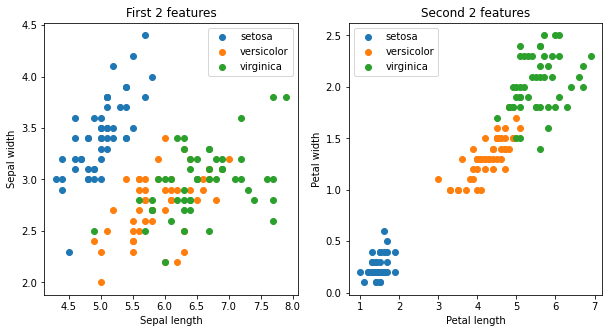
there are 4 features in the Iris data set. Depending on which set of features we use for visualization, we see the clusters separate more clearly.

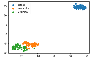
Let’s try using the tSNE method to visualize the data.

from sklearn.manifold import TSNE
model = TSNE(n_components=2, random_state=0)
X_transformed = model.fit_transform(X)
print(X.shape, X_transformed.shape)

(150, 4) (150, 2)

for name in iris.target_names:
    plt.scatter(X_transformed[y == name, 0], X_transformed[y == name, 1], label=name)
    
plt.legend()
plt.show()

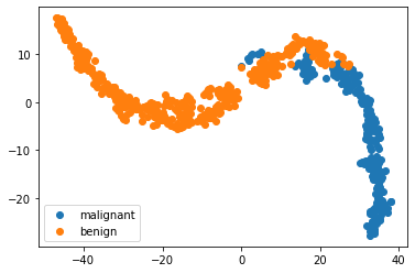
Lets take a look at the breast cancer dataset with dimensionality reduction

X = bc.data
y = bc.target_names[bc.target]
model = TSNE(n_components=2, random_state=1)
X_transformed = model.fit_transform(X)

for name in bc.target_names:
    plt.scatter(X_transformed[y == name, 0], X_transformed[y == name, 1], label=name)
    
plt.legend()

<matplotlib.legend.Legend at 0x7fba61eb5c70>

X_train, X_test, y_train, y_test = train_test_split(X, y, test_size=0.2, random_state=0)
model = KNeighborsClassifier()
model.fit(X_train, y_train)
print(metrics.classification_report(model.predict(X_test), y_test))

              precision    recall  f1-score   support

      benign       0.94      0.95      0.95        66
   malignant       0.94      0.92      0.93        48

    accuracy                           0.94       114
   macro avg       0.94      0.94      0.94       114
weighted avg       0.94      0.94      0.94       114

ypred = model.predict(X)
for name in bc.target_names:
    plt.scatter(X_transformed[ypred == name, 0], X_transformed[ypred == name, 1], label=name)
    
plt.legend()

<matplotlib.legend.Legend at 0x7fba6271b8e0>

previous

Pandas

next

Dimension Reduction and Data Visualization