Boundary Value Problems
Contents
Boundary Value Problems
In initial value problems, we find a unique solution to an ODE by specifying initial conditions. Another way to obtain a unique solution to an ODE (or PDE) is to specify boundary values.
The Heat Equation
The Heat Equation is a second-order PDE obeying
\begin{equation} \Delta u(x, t) = \partial_t u(x, t) \end{equation} where \(\Delta\) is the Laplacian operator \begin{equation} \Delta = \sum_i \partial_i^2 \end{equation}
This equation is in a steady state if \(\partial_t u = 0\) (i.e. the solution is not changing with time).
We’ll consider the steady state of the heat equation on a 1-dimensional domain \([0,1]\), where we have the ends of the domain set to fixed temperatures. In this case, we can write the solution as a boundary value problem for a second-order ODE: \begin{equation} \frac{d^2 u}{dx^2} = 0 \qquad u\in (0,1)\ u(0) = a\ u(1) = b \end{equation}
You might think of this as describing the temperature of a metal bar which is placed between two objects of differing temperatures.
import numpy as np
import scipy.linalg as la
import matplotlib.pyplot as plt
from scipy.integrate import solve_bvp
we’ll introduce the variable \(p = du / dx\) to obtain a system of first-order ODEs: \begin{equation} \frac{dp}{dx} = 0\ \frac{du}{dx} = p \end{equation}
with the same boundary conditions. The variable y = [u, p] will be a 2-vector containing the state.
We’ll use boundary conditions \(y(0)[0] = u(0) = 5 = a\) and \(y(1)[0] = u(1) = 1 = b\)
Finally, we use solve_bvp from scipy.integrate to solve the boundary value problem:
np.vstack((np.zeros(3), [3,4,5]))
array([[0., 0., 0.],
       [3., 4., 5.]])
a = 5
b = 1

def f(x, y):
    "right hand side of ODE"
    return np.vstack([y[1,:], np.zeros(y.shape[1])]) # du/dx = p, dp/dx = 0

def bc(y0, y1): # ya = y[:,0], yb = y[:,-1]
    "boundary condition residual"
    return np.array([y0[0] - a, y1[0] - b])

n = 100 # number of points
x = np.linspace(0,1,n)
# y0 = np.zeros((2,n))
y0 = np.random.randn(2,n)

# solve bvp
sol = solve_bvp(f, bc, x, y0)
we can plot the solution value
plt.plot(sol.x, sol.y[0,:])
plt.xlabel('x')
plt.ylabel('y')
plt.show()
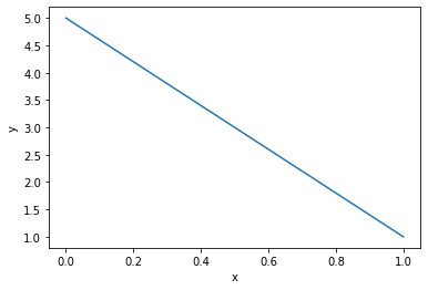
we see the solution is a linear function from (0,5) to (1,1). You can check that such a linear function solves the BVP mathematically.
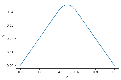
We also provide a non-zero right hand side: \(\partial_t u(x,t) = f(x)\).
def f(x, y):
    "right hand side of ODE"
    src = -1*np.logical_and(x < 0.6, x > 0.4)
    return np.vstack([y[1,:], src])

def bc(ya, yb):
    "boundary condition residual"
    return np.array([ya[0], yb[0]])

n = 100 # number of points
x = np.linspace(0,1,n)
y0 = np.zeros((2,n))

# solve bvp
sol = solve_bvp(f, bc, x, y0)

plt.plot(sol.x, sol.y[0,:])
plt.xlabel('x')
plt.ylabel('y')
plt.show()
/home/brad/miniconda3/envs/pycourse/lib/python3.8/site-packages/scipy/integrate/_bvp.py:1093: RuntimeWarning: invalid value encountered in true_divide
  r_middle = 1.5 * col_res / h
/home/brad/miniconda3/envs/pycourse/lib/python3.8/site-packages/scipy/integrate/_bvp.py:592: RuntimeWarning: invalid value encountered in true_divide
  slope = (y[:, 1:] - y[:, :-1]) / h
/home/brad/miniconda3/envs/pycourse/lib/python3.8/site-packages/scipy/integrate/_bvp.py:1103: RuntimeWarning: invalid value encountered in greater
  insert_1, = np.nonzero((rms_res > tol) & (rms_res < 100 * tol))
/home/brad/miniconda3/envs/pycourse/lib/python3.8/site-packages/scipy/integrate/_bvp.py:1103: RuntimeWarning: invalid value encountered in less
  insert_1, = np.nonzero((rms_res > tol) & (rms_res < 100 * tol))
/home/brad/miniconda3/envs/pycourse/lib/python3.8/site-packages/scipy/integrate/_bvp.py:1104: RuntimeWarning: invalid value encountered in greater_equal
  insert_2, = np.nonzero(rms_res >= 100 * tol)
The Wave Equation
The Wave Equation is another second order PDE obeying \begin{equation} \Delta u(x, t) = \partial_t^2 u(x, t) \end{equation}
One way to solve the Wave equaiton is to use separation of variables. This gives solutions of the form \begin{equation} u(x,t) = v(x) e^{i\omega t} \end{equation}
Where \(v(x)\) satisfies the Helmholtz equation \begin{equation} \Delta v(x) = -\omega^2 v(x) \end{equation}
In other words, \(v(x)\) is an eigenvector of the Laplacian operator with eigenvalue \(-\omega^2\). The time dependent portion of the solution \(e^{i\omega t}\) is simply a sinusoidal oscillation.
In a bounded domain, there is a discrete set of eigenvalues for the Laplacian. We’ll use the the construction \(\Delta = -\partial^T \partial\)
import scipy.sparse as sparse

# create matrix A to apply forward difference scheme
def forward_diff_matrix(n):
    data = []
    i = []
    j = []
    for k in range(n - 1):
        i.append(k)
        j.append(k)
        data.append(-1)

        i.append(k)
        j.append(k+1)
        data.append(1)

    # incidence matrix of the 1-d mesh
    return sparse.coo_matrix((data, (i,j)), shape=(n-1, n)).tocsr()

def Laplacian(n):
    """
    Create Laplacian on 1-dimensional grid with n nodes
    """
    B = forward_diff_matrix(n)
    return -B.T @ B
n = 100

x = np.linspace(0,1,n)
L = Laplacian(n)

L[:4,:4].todense()
matrix([[-1,  1,  0,  0],
        [ 1, -2,  1,  0],
        [ 0,  1, -2,  1],
        [ 0,  0,  1, -2]])
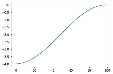
We can use the Gershgorin disk theorem to bound the eigenvalues in the range \([-4,0]\), or plot them experimentally:
lam, V = la.eigh(L.todense())
plt.plot(lam)
plt.show()
Let’s plot the eigenvectors with the 4 smallest-magnitude eigenvalues:
for i in range(1,5):
    plt.plot(x, V[:,-i], label=r"$v_{}$".format(i))

plt.legend()
plt.show()
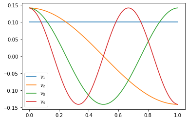
the eigenvectors are of the form \(v(x) = \cos(k \pi x)\) for \(k= 0,1,2,\dots\)
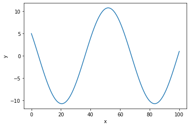
Now, let’s say we want to solve the boundary value problem \begin{equation} \Delta v = -\omega^2 v\ v[0] = a\qquad v[-1] = b \end{equation}
Again, we can use solve_bvp
a = 5
b = 1
omega = 0.1

def f(x, y):
    "right hand side of ODE"
    return np.vstack([y[1,:], -omega**2 * y[0,:]])

def bc(ya, yb):
    "boundary condition residual"
    return np.array([ya[0] - a, yb[0] - b])

n = 100 # number of points
x = np.linspace(0,n,n)
y0 = np.zeros((2,n))

# solve bvp
sol = solve_bvp(f, bc, x, y0)
plt.plot(sol.x, sol.y[0,:])
plt.xlabel('x')
plt.ylabel('y')
plt.show()
Boundary Value Problems in SymPy
SymPy offers functionality that can be used to solve BVPs in its sym.solvers.ode.dsolve function
import sympy as sym
from sympy.solvers import ode
x = sym.symbols('x') # symbol
u = sym.Function('u') # symbolic function
eqn = u(x).diff(x).diff(x) # = 0
eqn
ode.classify_ode(eqn)
('nth_algebraic',
 'nth_linear_constant_coeff_homogeneous',
 'nth_linear_euler_eq_homogeneous',
 'Liouville',
 '2nd_power_series_ordinary',
 'nth_algebraic_Integral',
 'Liouville_Integral')
ode.dsolve(eqn, hint='nth_linear_constant_coeff_homogeneous')
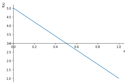
in order to pass in boundary conditions, you can use the ics parameter
f = ode.dsolve(eqn, hint='nth_linear_constant_coeff_homogeneous', ics={u(0): 5, u(1): 1})
f
sym.plot(f.rhs, (x, 0, 1))
<sympy.plotting.plot.Plot at 0x7f60d29d7b20>
Let’s try the Helmholtz equation now
omega = sym.Symbol('\omega')
eqn = u(x).diff(x).diff(x) + omega**2*u(x) # = 0
eqn
ode.classify_ode(eqn)
('nth_linear_constant_coeff_homogeneous', '2nd_power_series_ordinary')
ode.dsolve(eqn, hint='nth_linear_constant_coeff_homogeneous')
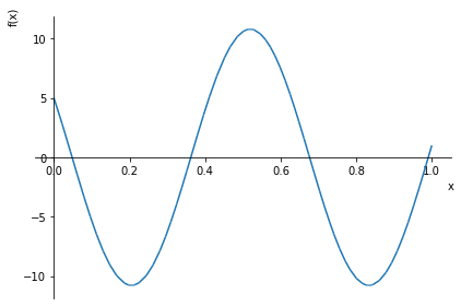
we see that the solution to the Helmholtz equation consists of sinusoidal waves. Let’s try putting in some boundary conditions
f = ode.dsolve(eqn, hint='nth_linear_constant_coeff_homogeneous', ics={u(0): 5, u(1): 1})
f
sym.plot(f.rhs.subs(omega, 10), (x, 0, 1))
<sympy.plotting.plot.Plot at 0x7f60d28616a0>
Solving BVPs using Optimization
You might also consider finding numerical solutions to BVPs using scipy.optimize. Let’s say we have a non-linear wave equation with boundary conditions
\begin{equation}
\Delta u = -f(u)\
u(x) = 0 \qquad x\in \partial \Omega
\end{equation}
where \(\partial \Omega\) is the boundary of the domain. We can seek to solve the optimization problem
\begin{equation}
\mathop{\mathsf{minimize}}_u |\Delta u + f(u)|\
\text{subject to } u(x) = 0 \qquad x \in \partial \Omega
\end{equation}
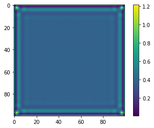
we’ll use \(f(u) = u^3\), modifying the example from the SciPy Cookbook
def interior_laplacian(n):
    """
    Laplacian defined on the interior a length n grid
    """
    L = Laplacian(n).todok()
    L[0,0] = 0
    L[1,0] = 0
    L[-1,-1] = 0
    L[-2,-1] = 0
    return L.tocsr()

def interior_eye(n):
    diag = np.ones(n)
    diag[0] = 0
    diag[-1] = 0
    In = sparse.dia_matrix((diag, 0), shape=(n,n))
    return In


def interior_laplacian_2d(m, n):
    """
    Laplacian defined on the interior of a m x n grid
    """
    Lm = interior_laplacian(m)
    Im = interior_eye(m)
    Ln = interior_laplacian(n)
    In = interior_eye(n)
    return sparse.kron(Lm, In) + sparse.kron(Im, Ln)
m = 100
n = 100
L = interior_laplacian_2d(m,n)

def rhs(u):
    return u**3

def f(u, *args, **kwargs):
    # return vector of residuals
    Lu = L @ u
    return Lu + rhs(u)
We’ll also define the jacobian
def compute_jac_indices(n):
    """
    compute indices for the Jacobian.  These are fixed for all iterations
    """
    i = np.arange(n)
    jj, ii = np.meshgrid(i, i)

    ii = ii.ravel()
    jj = jj.ravel()

    ij = np.arange(n**2)

    jac_rows = [ij]
    jac_cols = [ij]

    mask = ii > 0
    ij_mask = ij[mask]
    jac_rows.append(ij_mask)
    jac_cols.append(ij_mask - n)

    mask = ii < n - 1
    ij_mask = ij[mask]
    jac_rows.append(ij_mask)
    jac_cols.append(ij_mask + n)

    mask = jj > 0
    ij_mask = ij[mask]
    jac_rows.append(ij_mask)
    jac_cols.append(ij_mask - 1)

    mask = jj < n - 1
    ij_mask = ij[mask]
    jac_rows.append(ij_mask)
    jac_cols.append(ij_mask + 1)

    return np.hstack(jac_rows), np.hstack(jac_cols)


jac_rows, jac_cols = compute_jac_indices(100)


def jac(u, jac_rows=None, jac_cols=None):
    n = len(u)
    jac_values = np.ones_like(jac_cols, dtype=float)
    jac_values[:n] = -4 + 3*u**2
    return sparse.coo_matrix((jac_values, (jac_rows, jac_cols)), shape=(n, n))
import scipy.optimize as opt


res = opt.least_squares(
    f,
    # np.random.rand(m*n),
    np.ones(m*n),
    jac=jac,
    kwargs={'jac_rows': jac_rows, 'jac_cols': jac_cols},
    verbose=1)
`xtol` termination condition is satisfied.
Function evaluations 27, initial cost 5.3960e+03, final cost 5.3860e+01, first-order optimality 1.15e+00.
xsol = np.reshape(res.x, (100,100))

plt.imshow(xsol)
plt.colorbar()
plt.show()