Basic Containers and Packages
Contents
Basic Containers and Packages
Python Lists
Lists are a data structure provided as part of the Python language. Lists and more on lists..
A list is compound data type which is a mutable, indexed, and ordered collection of data.
Lists are often constructed using square brackets: [...]
x0 = [1, 2, 3] # list of numbers
print(x0)
print(type(x0))
[1, 2, 3]
<class 'list'>
x1 = ['hello', 'world'] # list of strings
print(x1)
print(type(x1))
['hello', 'world']
<class 'list'>
x = [x0, x1] # list of lists
print(x)
print(type(x))
[[1, 2, 3], ['hello', 'world']]
<class 'list'>
Usually lists will be generated programatically. One way you can do this is by using the append method
x = [] # empty list
for i in range(5):
    x.append(i)
x
[0, 1, 2, 3, 4]
or the extend method, which appends all elements in another list
x = [1,2,3]
y = [4,5,6]
x.extend(y) # extends x by y
x
[1, 2, 3, 4, 5, 6]
you can also extend lists using the + operator
[1,2,3] + [4,5,6]
[1, 2, 3, 4, 5, 6]
You can also generate lists using list comprehensions. Comprehensions are “Pythonic” which is a vauge term roughly meaning
Pythonic: “something a Python programmer would write”
x = [i for i in range(5)]
x
[0, 1, 2, 3, 4]
x = [i * i for i in range(5)]
x
[0, 1, 4, 9, 16]
Generally, comprensions consist of [expression loop conditional]
This looks a lot like set notation in mathematics. E.g. for the set $\(y = \{i \mid i \in x, i \ne 4\}\)$ we compute
y = [i for i in x if i != 4]
y
[0, 1, 9, 16]
Indexing
Python is 0-indexed (like C, unlike fortran/Matlab). This means a list of length n will have indices that start at 0, and end at n-1.
This is the reason why range(n) iterates through the range 0,...,n-1
words = ["dog", "cat", "house"]
print(words[0])
print(words[1])
dog
cat
you can access elements starting at the back of the array using negative integers. A good way to think of this is the index -1 translates to n-1
print(words[-1])
print(words[-2])
house
cat
Slicing - you can use the colon character : to slice an array. The syntax is start:end:stride
x = [i for i in range(10)]
print(x)
print(x[:])
print(x[2:4])
print(x[2:9:3])
print(x[-3:-1])
print(x[::2])
print(x[::-1])
[0, 1, 2, 3, 4, 5, 6, 7, 8, 9]
[0, 1, 2, 3, 4, 5, 6, 7, 8, 9]
[2, 3]
[2, 5, 8]
[7, 8]
[0, 2, 4, 6, 8]
[9, 8, 7, 6, 5, 4, 3, 2, 1, 0]
Lists are mutable, which means you can change elements
words = ["dog", "cat", "house"]
print(words)

words[0] = "mouse"
print(words)
['dog', 'cat', 'house']
['mouse', 'cat', 'house']
Other Python Collections
There are other collections you might use in Python:
Tuples
(...)are ordered, indexed, and immutableSets
{...}are unordered, unindexed, and mutableDictionaries
{...}are unordered, indexed, and mutable
These collections also support comprehensions.
You can find additional types of collections in the Collections module
x = (1,2,3) # tuple
print(x)
x = (i for i in range(1,4)) # tuple comprehension
print(tuple(x))
(1, 2, 3)
(1, 2, 3)
s = {1,2,3} # set
1 in s
True
s = {i for i in range(1,4)}
s
{1, 2, 3}
d = {'hello' : 0, 'goodbye': 1} # dictionary
print(type(d))
d['hello']
<class 'dict'>
0
d = {key: val for val, key in enumerate(['hello', 'goodbye'])}
d
{'hello': 0, 'goodbye': 1}
Numpy
If you haven’t already:
conda install numpy
Numpy is perhaps the fundamental scientific computing package for Python - just about every other package for scientific computing uses it.
Numpy basically provides a ndarray type (n-dimensional array), and provides fast operations for arrays (i.e. compiled C or Fortran).
We’ll do some deeper dives into numpy in future lectures. For now, we’ll cover some basics. For those who want to dive in now, here are some tutorials
Quickstart Tutorial - for those with more experience in other languages
You can find lots of information in the numpy documentation
import numpy as np # import numpy into the np namespace
You can easily generate numpy arrays from list data
x = np.array([1,2,3])
print(x)
print(type(x))
[1 2 3]
<class 'numpy.ndarray'>
A 2-dimensional array can be generated by lists of lists
x = np.array([[1,2,3], [4,5,6]])
print(x)
[[1 2 3]
 [4 5 6]]
a few class members:
print(x.ndim) # number of dimensions
print(x.shape) # shape of array
print(x.size) # total number of elements in array
print(x.dtype) # data type
print(x.itemsize) # number of bytes for data type
print(x.data) # buffer location in memory
print(x.flags) # some flags
2
(2, 3)
6
int64
8
<memory at 0x7f52bcf60e10>
  C_CONTIGUOUS : True
  F_CONTIGUOUS : False
  OWNDATA : True
  WRITEABLE : True
  ALIGNED : True
  WRITEBACKIFCOPY : False
  UPDATEIFCOPY : False
Other ways of obtaining numpy arrays:
# array from a range
a = np.arange(3)
print(a)

# an array of 1
a = np.ones((3,2), dtype=np.float)
print(a)

# just an array with no initialization - WARNING: data can be anything
a = np.empty((3,2), dtype=np.float)
print(a)

# random normal data
a = np.random.normal(size=(3,2))
print(a)
[0 1 2]
[[1. 1.]
 [1. 1.]
 [1. 1.]]
[[1. 1.]
 [1. 1.]
 [1. 1.]]
[[-0.02886968 -0.28269196]
 [-0.48312791 -0.3424373 ]
 [ 0.25438968  0.29092363]]
Indexing
1-dimensional arrays are indexed in the same way as lists (0-indexed, can use slices, etc)
a = np.arange(4)
print(a[:2])
[0 1]
you can also index using lists of indices
inds = [0,2]
a[inds]
array([0, 2])
2-dimensional arrays are a bit different from lists of lists:
a = [[0,1],[2,3]] # list of lists
print(a)
a[1][1] # like indexing in C
[[0, 1], [2, 3]]
3
anp = np.array(a) # 2-dimensional array
anp[1,1] # like indexing in Matlab, Julia
3
you can also use slices, index sets, etc. in multi-dimensional arrays.
If you only provide 1 index, you’ll get the corresponding row (or set of rows if slicing)
anp[0]
array([0, 1])
Arithmetic
Numpy arrays support basic element-wise arithmetic, assuming arrays are the same shape.
Note: there are more complicated broadcasting rules for different-shaped arrays, which we’ll cover some other time.
x = np.arange(4)
print(x)
print(x + x)
print(x * x)
print(x**3)

def f(x):
    return x**2 - 2*x + 1

print(f(x))
[0 1 2 3]
[0 2 4 6]
[0 1 4 9]
[ 0  1  8 27]
[1 0 1 4]
Warning: The * operator applied to 2-dimensional arrays is not the same as matrix-matrix multiplication. It will perform element-wise multiplication instead.
Numpy provides the @ operator for matrix multiplication. You can also use the matmul() or dot() (dot product) methods.
x = np.arange(4).reshape(2,2)
print(x)
print(x*x)
print(x @ x)
print(x.dot(x))
print(np.matmul(x,x))
[[0 1]
 [2 3]]
[[0 1]
 [4 9]]
[[ 2  3]
 [ 6 11]]
[[ 2  3]
 [ 6 11]]
[[ 2  3]
 [ 6 11]]
Numpy provides a variety of mathematics functions that you can use with numpy arrays. Numpy is vectorized, meaning that it is typically much faster to perform array operations than to use explicit for loops. This should be a familiar concept to Matlab users.
np.sin(x)
array([[0.        , 0.84147098],
       [0.90929743, 0.14112001]])
import time
n = 1_000_000
# list data
x = [i/n for i in range(n)]
# numpy array
xnp = np.array(x)

# square elements in-place
t0 = time.monotonic()
for i in range(n):
    x[i] = x[i] * x[i]
t1 = time.monotonic()
print("time for loop over list: {:.3} sec.".format(t1 - t0))

t0 = time.monotonic()
xnp = xnp * xnp
t1 = time.monotonic()
print("time for numpy vectorization: {:.3} sec.".format(t1 - t0))
time for loop over list: 0.147 sec.
time for numpy vectorization: 0.00184 sec.
PyPlot
PyPlot is a go-to plotting tool for Python. It is fully operable with numpy arrays.
conda install matplotlib
import matplotlib.pyplot as plt
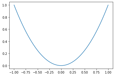
# plot a single function
x = np.linspace(-1,1,100)
y = x * x
plt.plot(x,y)
plt.show()
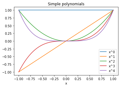
# plot multiple functions
x = np.linspace(-1,1,100)
for n in range(5):
    plt.plot(x,x**n, label=f"x^{n}")
plt.legend()
plt.xlabel("x")
plt.title("Simple polynomials")
plt.show()
CSV files, Pandas
The *.csv extension is typically used to denote a “comma seperated value” file. These types of files are often used to store arrays in human-readable plain text.
Here’s an example:
0, 1, 2, 3
4, 5, 6, 7
...
You can save numpy arrays to files using np.savetxt()
# generates example.csv
n = 1000
x = np.arange(4*n).reshape(-1,4)
np.savetxt("example.csv", x, fmt="%d", delimiter=',')
Files can be loaded using np.loadtxt()
y = np.loadtxt('example.csv', dtype=np.int, delimiter=',')
y
array([[   0,    1,    2,    3],
       [   4,    5,    6,    7],
       [   8,    9,   10,   11],
       ...,
       [3988, 3989, 3990, 3991],
       [3992, 3993, 3994, 3995],
       [3996, 3997, 3998, 3999]])
Often, scientific data has some meaning associated with numbers. In this case, the csv file might have a header, and every row is a different data point.
temperature, density, width, length
0, 1, 2, 3
4, 5, 6, 7
...
You can still load using numpy, but it is easy to loose track of what the different columns of the array mean.
The solution for this sort of data is to use a Pandas dataframe
conda install pandas
import pandas as pd
data = pd.read_csv('example.csv', header=None, sep=',')
data
| 0 | 1 | 2 | 3 | |
|---|---|---|---|---|
| 0 | 0 | 1 | 2 | 3 |
| 1 | 4 | 5 | 6 | 7 |
| 2 | 8 | 9 | 10 | 11 |
| 3 | 12 | 13 | 14 | 15 |
| 4 | 16 | 17 | 18 | 19 |
| ... | ... | ... | ... | ... |
| 995 | 3980 | 3981 | 3982 | 3983 |
| 996 | 3984 | 3985 | 3986 | 3987 |
| 997 | 3988 | 3989 | 3990 | 3991 |
| 998 | 3992 | 3993 | 3994 | 3995 |
| 999 | 3996 | 3997 | 3998 | 3999 |
1000 rows × 4 columns
# this will set the header identitites and save the file
data = pd.read_csv('example.csv', header=None, names=["temperature", "density", "width", "length"])
data.to_csv("example2.csv", index=False) # writes to csv with headers
data
| temperature | density | width | length | |
|---|---|---|---|---|
| 0 | 0 | 1 | 2 | 3 |
| 1 | 4 | 5 | 6 | 7 |
| 2 | 8 | 9 | 10 | 11 |
| 3 | 12 | 13 | 14 | 15 |
| 4 | 16 | 17 | 18 | 19 |
| ... | ... | ... | ... | ... |
| 995 | 3980 | 3981 | 3982 | 3983 |
| 996 | 3984 | 3985 | 3986 | 3987 |
| 997 | 3988 | 3989 | 3990 | 3991 |
| 998 | 3992 | 3993 | 3994 | 3995 |
| 999 | 3996 | 3997 | 3998 | 3999 |
1000 rows × 4 columns
data2 = pd.read_csv("example2.csv") # read csv with headers
data2
| temperature | density | width | length | |
|---|---|---|---|---|
| 0 | 0 | 1 | 2 | 3 |
| 1 | 4 | 5 | 6 | 7 |
| 2 | 8 | 9 | 10 | 11 |
| 3 | 12 | 13 | 14 | 15 |
| 4 | 16 | 17 | 18 | 19 |
| ... | ... | ... | ... | ... |
| 995 | 3980 | 3981 | 3982 | 3983 |
| 996 | 3984 | 3985 | 3986 | 3987 |
| 997 | 3988 | 3989 | 3990 | 3991 |
| 998 | 3992 | 3993 | 3994 | 3995 |
| 999 | 3996 | 3997 | 3998 | 3999 |
1000 rows × 4 columns
You can get columns of a dataframe by using the column label
data2['temperature']
0         0
1         4
2         8
3        12
4        16
       ...
995    3980
996    3984
997    3988
998    3992
999    3996
Name: temperature, Length: 1000, dtype: int64
To get rows, use the iloc parameter:
data2.iloc[1:3]
| temperature | density | width | length | |
|---|---|---|---|---|
| 1 | 4 | 5 | 6 | 7 |
| 2 | 8 | 9 | 10 | 11 |
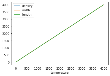
You can easily plot labeled columns
data.plot('temperature')
plt.show()