PyTorch Neural Networks
Contents
PyTorch Neural Networks
PyTorch is a Python package for defining and training neural networks. Neural networks and deep learning have been a hot topic for several years, and are the tools underlying many state-of-the art machine learning tasks. There are many industrial applications (e.g. at your favorite or least favorite companies in Silicon Valley), but also many scientific applications including
Processing data in particle detectors
Seismic imaging / medical imaging
Accelerating simulations of physical phenomena
…
A (deep) feed-forward neural network is the composition of functions \begin{equation} f_N(x; w_N, b_N) \circ f_{N-1}(x; w_{N-1}, b_{N-1}) \circ \dots f_0(x; w_0, b_0) \end{equation} where each \(f_i(x; w_i, b_i)\) is a (non-linear) function with learnable parameters \(w_i, b_i\). There are many choices for what the exact function is. A common and simple one to describe is an (affine) linear transformation followed by a non-linearity. \begin{equation} f_i(x; w_i, b_i) = (w_i \cdot x + b_i)_+ \end{equation}
where \(w_i \cdot x\) is matrix-vector multiplication, and \((\cdot)_+\) is the ReLU operation (Rectified Linear Unit) \begin{equation} x_+ = \begin{cases} x & x > 0\ 0 & x \le 0 \end{cases} \end{equation}
If you take the composition of several functions like this, you have a multilayer perceptron (MLP).
Deep Learning Libraries
There are many deep learning libraries available, the most common ones for python are
TensorFlow, Keras
PyTorch
Working with tensorflow requires going into lot of details of the contruction of the computation graph, whereas Keras is a higher level interface for tensorflow. Tensorflow is very popular in the industry and good for production code.
PyTorch can be used as low level interface, but is much more user-friendly than tensorflow, but it also has a higher level interface. Pytorch is more popular in the research community.
Main features that any deep learning library should provide
No matter what library or language you use, the main features provided by a deep learning library are
Use the GPU to speed up computation
Ability to do automatic differentiation
Useful library functions for common architectures and optimization algorithms
PyTorch
We will look at all of the above in pytorch. The best way to think about pytorch is that its numpy + GPU + autograd.
You can install it with
conda install pytorch.
Alternatively (and recommended), run this notebook in Google Colab– it provides an environment with all of the PyTorch dependencies plus a GPU free of charge.
import torch
import numpy as np
import matplotlib.pyplot as plt
torch.__version__
'1.7.0'
Automatic Differentiation
Automatic differentiation is different from numerical differentiation, which requires a choice of step size, and symbolic differentiation which creates a single expression for a derivative. Instead it performs chain rule repeatedly.
PyTorch uses dynamic computation graphs to compute the gradients of the parameters.
x = torch.tensor([2.0])
m = torch.tensor([5.0], requires_grad = True)
c = torch.tensor([2.0], requires_grad = True)
y = m*x + c
y
tensor([12.], grad_fn=<AddBackward0>)
Define an error for your function
loss = torch.norm( y - 13)
loss
tensor(1., grad_fn=<CopyBackwards>)
m.grad
Calling x.backward() on any tensor forces pytorch to compute all the gradients of the tensors used to compute x which had the requires_grad flag set to True. The computed gradient will be stored in the .grad property of the tensors
loss.backward()
m.grad
tensor([-2.])
c.grad
tensor([-1.])
with torch.no_grad():
    m -= 0.01 * m.grad
    c -= 0.3 * c.grad
m,c
(tensor([5.0200], requires_grad=True), tensor([2.3000], requires_grad=True))
m.grad, c.grad
(tensor([-2.]), tensor([-1.]))
m.grad.zero_()
c.grad.zero_()

m.grad, c.grad
(tensor([0.]), tensor([0.]))
y = m*x + c
y
tensor([12.3400], grad_fn=<AddBackward0>)
loss = torch.norm( y - 13)
loss
tensor(0.6600, grad_fn=<CopyBackwards>)
loss.backward()
m.grad, c.grad
(tensor([-2.]), tensor([-1.]))
Making it more compact
def model_fn(x,m,c):
    return m*x + c

def loss_fn(y,yt):
    return torch.norm(y-yt)
m = torch.tensor([5.0], requires_grad = True)
c = torch.tensor([2.0], requires_grad = True)
x = torch.tensor([2.0])
yt = torch.tensor([13.0])
y = model_fn(x,m,c)
loss = loss_fn(y,yt)
loss.backward()
with torch.no_grad():
    m -= 0.05 * m.grad
    c -= 0.05 * c.grad
m.grad.zero_()
c.grad.zero_()

print( f" m = {m}\n c = {c}\n y = {y}\n loss = {loss}")
#note that 'loss' indicates the loss for the previous m,c values
 m = tensor([5.1000], requires_grad=True)
 c = tensor([2.0500], requires_grad=True)
 y = tensor([12.], grad_fn=<AddBackward0>)
 loss = 1.0
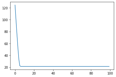
Here’s an explicit loop:
x = torch.randn(5,100)
yt = torch.randn(1,100)
losses = []

for i in range(100):
    y = model_fn(x,m,c)
    loss = loss_fn(y,yt)
    loss.backward()
    with torch.no_grad():
        m -= 0.05 * m.grad
        c -= 0.05 * c.grad
    m.grad.zero_()
    c.grad.zero_()

    losses+=[loss.item()]
    print( f"loss = {loss}")

plt.plot(losses);
loss = 124.58647155761719
loss = 100.0760726928711
loss = 76.15535736083984
loss = 53.43391036987305
loss = 33.741756439208984
loss = 22.521928787231445
loss = 21.386093139648438
loss = 21.377168655395508
loss = 21.376569747924805
loss = 21.37651824951172
loss = 21.376510620117188
loss = 21.376516342163086
loss = 21.37651252746582
loss = 21.376514434814453
loss = 21.376508712768555
loss = 21.376506805419922
loss = 21.376508712768555
loss = 21.376510620117188
loss = 21.376510620117188
loss = 21.376510620117188
loss = 21.376510620117188
loss = 21.376510620117188
loss = 21.376510620117188
loss = 21.376510620117188
loss = 21.376510620117188
loss = 21.376510620117188
loss = 21.376510620117188
loss = 21.376510620117188
loss = 21.376510620117188
loss = 21.376510620117188
loss = 21.376510620117188
loss = 21.376510620117188
loss = 21.376510620117188
loss = 21.376510620117188
loss = 21.376510620117188
loss = 21.376510620117188
loss = 21.376510620117188
loss = 21.376510620117188
loss = 21.376510620117188
loss = 21.376510620117188
loss = 21.376510620117188
loss = 21.376510620117188
loss = 21.376510620117188
loss = 21.376510620117188
loss = 21.376510620117188
loss = 21.376510620117188
loss = 21.376510620117188
loss = 21.376510620117188
loss = 21.376510620117188
loss = 21.376510620117188
loss = 21.376510620117188
loss = 21.376510620117188
loss = 21.376510620117188
loss = 21.376510620117188
loss = 21.376510620117188
loss = 21.376510620117188
loss = 21.376510620117188
loss = 21.376510620117188
loss = 21.376510620117188
loss = 21.376510620117188
loss = 21.376510620117188
loss = 21.376510620117188
loss = 21.376510620117188
loss = 21.376510620117188
loss = 21.376510620117188
loss = 21.376510620117188
loss = 21.376510620117188
loss = 21.376510620117188
loss = 21.376510620117188
loss = 21.376510620117188
loss = 21.376510620117188
loss = 21.376510620117188
loss = 21.376510620117188
loss = 21.376510620117188
loss = 21.376510620117188
loss = 21.376510620117188
loss = 21.376510620117188
loss = 21.376510620117188
loss = 21.376510620117188
loss = 21.376510620117188
loss = 21.376510620117188
loss = 21.376510620117188
loss = 21.376510620117188
loss = 21.376510620117188
loss = 21.376510620117188
loss = 21.376510620117188
loss = 21.376510620117188
loss = 21.376510620117188
loss = 21.376510620117188
loss = 21.376510620117188
loss = 21.376510620117188
loss = 21.376510620117188
loss = 21.376510620117188
loss = 21.376510620117188
loss = 21.376510620117188
loss = 21.376510620117188
loss = 21.376510620117188
loss = 21.376510620117188
loss = 21.376510620117188
loss = 21.376510620117188
Using Library functions
The subpackage torch.nn provides an object-oriented library of functions that can be composed together.
model = torch.nn.Sequential(
    torch.nn.Linear(5, 5), # 5 x 5 matrix
    torch.nn.ReLU(),       # ReLU nonlinearity
    torch.nn.Linear(5, 5), # 5 x 5 matrix
)
list(model.parameters())
[Parameter containing:
 tensor([[ 0.0149,  0.3121,  0.2289,  0.3779, -0.3541],
         [ 0.2562, -0.3695, -0.3553, -0.1636, -0.2496],
         [-0.2948,  0.3897, -0.3160, -0.0184,  0.0073],
         [ 0.0915, -0.3623, -0.4183, -0.1774,  0.0796],
         [ 0.0279, -0.4043, -0.3383,  0.1285,  0.4144]], requires_grad=True),
 Parameter containing:
 tensor([-0.3120,  0.1994, -0.4026,  0.0500,  0.3989], requires_grad=True),
 Parameter containing:
 tensor([[-0.2343, -0.1922,  0.2610, -0.3042, -0.0153],
         [-0.2047, -0.3752,  0.1721, -0.3577, -0.3788],
         [ 0.0965, -0.1811,  0.0690, -0.3732,  0.3016],
         [-0.1894,  0.0812, -0.1556, -0.0575, -0.4400],
         [-0.2093,  0.0431,  0.1603,  0.1434, -0.1087]], requires_grad=True),
 Parameter containing:
 tensor([-0.0123,  0.3197, -0.4355,  0.1170,  0.3940], requires_grad=True)]
loss_fn = torch.nn.MSELoss(reduction='sum')
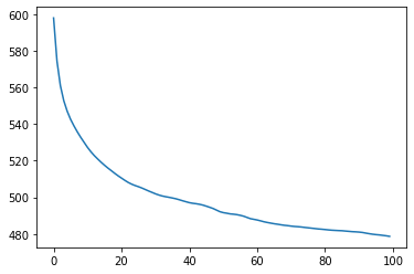
In this case, we’ll just fit the model to random data.
x = torch.randn(100,5)
yt = torch.randn(100,5)
losses = []
Optimizers in torch.optim implement a variety of optimization strategies. Almost all are based on gradient descent, since forming Hessians is prohibitive.
optimizer = torch.optim.Adam(model.parameters(), lr=0.03)
for i in range(100):
    y = model(x)
    loss = loss_fn(y,yt)
    loss.backward()

    optimizer.step()
    optimizer.zero_grad()

    losses+=[loss.item()]
    print( f"loss = {loss}")

plt.plot(losses);
loss = 597.9461669921875
loss = 574.3831787109375
loss = 560.9655151367188
loss = 552.7423095703125
loss = 547.044677734375
loss = 542.5809326171875
loss = 538.9766845703125
loss = 535.6971435546875
loss = 532.70849609375
loss = 529.9525146484375
loss = 527.230224609375
loss = 524.8335571289062
loss = 522.7387084960938
loss = 520.8978271484375
loss = 519.1264038085938
loss = 517.4871826171875
loss = 515.9583740234375
loss = 514.5322265625
loss = 513.0758666992188
loss = 511.7215576171875
loss = 510.4723205566406
loss = 509.22216796875
loss = 508.0721740722656
loss = 507.1442565917969
loss = 506.3977966308594
loss = 505.76324462890625
loss = 505.0520935058594
loss = 504.23699951171875
loss = 503.42218017578125
loss = 502.65570068359375
loss = 501.8807373046875
loss = 501.22955322265625
loss = 500.6920166015625
loss = 500.2988586425781
loss = 499.9666748046875
loss = 499.5892639160156
loss = 499.18121337890625
loss = 498.6595458984375
loss = 498.08392333984375
loss = 497.55181884765625
loss = 497.0421142578125
loss = 496.69696044921875
loss = 496.461669921875
loss = 496.1409606933594
loss = 495.70648193359375
loss = 495.125
loss = 494.5040283203125
loss = 493.8422546386719
loss = 492.9754333496094
loss = 492.11651611328125
loss = 491.59033203125
loss = 491.2809143066406
loss = 490.9151916503906
loss = 490.73663330078125
loss = 490.4977722167969
loss = 490.1248779296875
loss = 489.64532470703125
loss = 488.96630859375
loss = 488.28997802734375
loss = 487.94036865234375
loss = 487.5657653808594
loss = 487.0981140136719
loss = 486.5963134765625
loss = 486.2052917480469
loss = 485.85565185546875
loss = 485.5244140625
loss = 485.2522888183594
loss = 484.9501037597656
loss = 484.6748962402344
loss = 484.4850158691406
loss = 484.23541259765625
loss = 484.03240966796875
loss = 483.9110107421875
loss = 483.74169921875
loss = 483.5115051269531
loss = 483.3094482421875
loss = 483.09991455078125
loss = 482.889892578125
loss = 482.68017578125
loss = 482.531982421875
loss = 482.34814453125
loss = 482.1547546386719
loss = 481.9912109375
loss = 481.884521484375
loss = 481.7872314453125
loss = 481.70562744140625
loss = 481.52581787109375
loss = 481.36749267578125
loss = 481.2004089355469
loss = 481.10504150390625
loss = 480.96807861328125
loss = 480.7559509277344
loss = 480.4117431640625
loss = 480.0869140625
loss = 479.7966613769531
loss = 479.5823059082031
loss = 479.4156494140625
loss = 479.1708068847656
loss = 478.93817138671875
loss = 478.64166259765625
MNIST Example
First, you’ll want to install the torchvision package - this is a package for PyTorch that provides a variety of computer vision functionality.
The MNIST data set consists of a collection of handwritten digits (0-9). Our goal is to train a neural net which will classify the image of each digit as the correct digit
conda install torchvision -c pytorch
import torchvision
from torchvision.datasets import MNIST
data = MNIST(".",download=True)
len(data)
60000
import numpy as np
img,y = data[np.random.randint(1,60000)]
print(y)
img
7

data.train_data[2].shape
/home/brad/miniconda3/envs/pycourse/lib/python3.8/site-packages/torchvision/datasets/mnist.py:58: UserWarning: train_data has been renamed data
  warnings.warn("train_data has been renamed data")
torch.Size([28, 28])
data.train_labels[2]
/home/brad/miniconda3/envs/pycourse/lib/python3.8/site-packages/torchvision/datasets/mnist.py:48: UserWarning: train_labels has been renamed targets
  warnings.warn("train_labels has been renamed targets")
tensor(4)
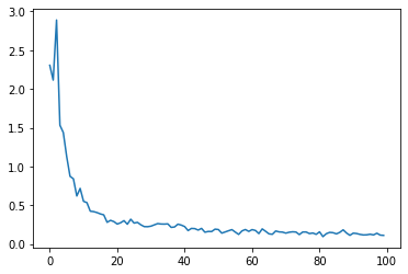
MNIST Training
model = torch.nn.Sequential(
    torch.nn.Linear(784, 100),
    torch.nn.ReLU(),
    torch.nn.Linear(100, 100),
    torch.nn.ReLU(),
    torch.nn.Linear(100, 10),
)
loss_fn = torch.nn.CrossEntropyLoss()
sample = np.random.choice(range(len(data.train_data)),1000)
x = data.train_data[sample].reshape(1000,-1).float()/255
yt = data.train_labels[sample]
x.shape,yt.shape
(torch.Size([1000, 784]), torch.Size([1000]))
optimizer = torch.optim.Adam(model.parameters(), lr=0.03)
losses = []
for i in range(100):

    sample = np.random.choice(range(len(data.train_data)),1000)
    x = data.train_data[sample].reshape(1000,-1).float()/255
    yt = data.train_labels[sample]

    y = model(x)
    loss = loss_fn(y,yt)
    loss.backward()

    optimizer.step()
    optimizer.zero_grad()

    losses+=[loss.item()]
    #print( f"loss = {loss}")
plt.plot(losses);
x_test = data.train_data[-1000:].reshape(1000,-1).float()/255
y_test = data.train_labels[-1000:]
with torch.no_grad():
    y_pred = model(x_test)
print("Accuracy = ", (y_pred.argmax(dim=1) == y_test).sum().float().item()/1000.0)
Accuracy = 0.979
Credits
This notebook was adapted from a notebook from CME 193 at Stanford