Asymptotic Notation¶

First, let’s review some asymptotic notation. We’ll see it a fair amount in this course.

Let $f(x), g(x)$ be some functions. We say $$f = O(g)$$ as $x\to \infty$ if there exists some constant $c\ge 0$ and $x_0\ge 0$ so that $ |f(x)| \le c g(x)$ for all $x \ge x_0$.

We say $$f = \Omega(g)$$ as $x\to \infty$ if there exists some constant $c\ge 0$ and $x_0\ge 0$ so that $ |f(x)| \ge c g(x)$ for all $x \ge x_0$.

Finally, $$f = \Theta(g)$$ if $f = O(g)$ and $f = \Omega(g)$ (some constant multiples of $g$ bound $f$ above and below).

Often we’re interested in bounding worst-case behavior. This means you’ll see a lot of $O$, and less of $\Omega$ and $\Theta$.

You may also see little-o notation such as $f = o(g)$, or the corresponding $f = \omega(g)$. In these cases the inequalities are strict. If $f = o(g)$, then for any $c > 0$, there exists an $x_0\ge 0$ so that $|f(x)| < c g(x)$ for $x\ge x_0$. If $f = O(g)$ it can grow at the same rate, but if $f = o(g)$, it grows at a slower rate.

Note that because we can scale by constant multiples, we typically drop them.

$O(5x) = O(x)$
$O(c) = O(1)$
$O(c f(x)) = O(f(x))$

Examples¶

$x = O(x)$
$x = O(x^2)$
$x^a = O(x^b)$ for $a \le b$
$x^a = O(b^x)$ for any $a, b > 1$
$f = O(g)$ and $g = O(h)$ implies $f = O(h)$ (exercise: prove this)
$f = O(g)$ and $h = O(k)$ implies $f\times h = O(g \times k)$ (exercise: prove this as well)

Answers to example 5 and 6¶

Answer to example 5:

By definition, since $f = O(g)$, we know there exists some constant $p\ge 0$ and $x_0\ge 0$ so that $ |f(x)| \le p g(x)$ for all $x \ge x_0$; since $g = O(h)$, we know there exists some constant $q\ge 0$ and $x_1\ge 0$ so that $ |g(x)| \le q h(x)$ for all $x \ge x_1$. Therefore, we get $ |f(x)| \le p g(x)$ $ \le (p*q) h(x)$ as $x \ge $ $max$ {$x_0$, $x_1$}, which implies $f = O(h)$.

Answer to example 6: Still, by definition, since $f = O(g)$, we know there exists some constant $p\ge 0$ and $x_0\ge 0$ so that $ |f(x)| \le p g(x)$ for all $x \ge x_0$; since $h = O(k)$, we know there exists some constant $q\ge 0$ and $x_1\ge 0$ so that $ |h(x)| \le q k(x)$ for all $x \ge x_1$. Now, take $x'$ = $max$ {$x_0$, $x_1$}, we know as $x\ge x'$, we have both $ |f(x)| \le p g(x)$ and $ |h(x)| \le q k(x)$. Therefore, now we have: $|(f\times h) (x)| \le |f(x)| * |h(x)| \le (p*q) g(x) k(x) = (p*q) (g\times k) (x)$, proved.

Complexity¶

When we talk about computational complexity, we are typically talking about the time or memory resources needed for an algorithm.

For example, if an algorithm operates on an array of $n$ elements, we say the algorithm runs in $O(n^2)$ time if the run time scales (at worst) quadratically with the size $n$.

For example, consider the following function:

import numpy as np

def maximum(x):
    """
    returns the maximum value in an array x
    """
    xmax = -np.infty
    for xi in x:
        if xi > xmax:
            xmax = xi
            
    return xmax

maximum([1,3,2])

our maximum function loops over the list once, and at each step of the iteration we do a constant amount of work. If maximum takes in an array of length n as input, this means there are n iterations of the for-loop, so maximum takes $O(n)$ time to compute. Note that we don’t need to create any additional arrays, so we can also say maximum uses $O(1)$ (constant) extra space.

import matplotlib.pyplot as plt
from time import time

ns = [10**k for k in range(1,8)]
ts = []
for n in ns:
    a = np.random.rand(n)
    start = time()
    amax = maximum(a)
    end = time()
    ts.append(end - start)
    
plt.loglog(ns, ts)
plt.xlabel('n')
plt.ylabel('time (sec.)')
plt.title('time to compute maximum')
plt.show()

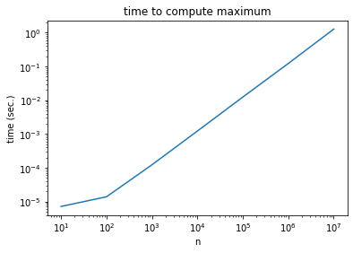
When plotting functions with polynomial complexity ($O(x^a)$ for some $a$), it is standard to use a loglog plot.

Why? If $t(n) = \Theta(n^a)$, then \begin{align*} t(n) &\sim c n^a\ \log t(n) &\sim a \log n + \log c \end{align*}

I.e. the polynomial exponent is the slope of the line.

ln = np.log(ns)
lt = np.log(ts)
coeff = np.polyfit(ln, lt, 1) # fit a polynomial
coeff[0] # highest degree (linear) term

0.916227608045119

Let’s now consider the following function

def all_subarrays(x):
    """
    return all sub-arrays of x
    """
    if len(x) == 1:
        return [x, []]
    else:
        ret = []
        subs = all_subarrays(x[:-1]) # subarrays with all but the last element
        ret.extend(subs) # all subarrrays without the last element
        for s in subs:
            scpy = s.copy()
            scpy.append(x[-1])
            ret.append(scpy)
        return ret
        
all_subarrays([0,1,2])

[[0], [], [0, 1], [1], [0, 2], [2], [0, 1, 2], [1, 2]]

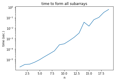
we see that the length of output of all_subarrays grows as $2^n$, where n = len(x). This is a good hint that the function has exponential time complexity and space complexity $O(2^n)$.

ns = range(1, 20)
ts = []
for n in ns:
    a = [i for i in range(n)]
    start = time()
    ret = all_subarrays(a)
    end = time()
    ts.append(end - start)

In this case, it is better to use a semilogy plot.

plt.semilogy(ns, ts)
plt.xlabel('n')
plt.ylabel('time (sec.)')
plt.title('time to form all subarrays')
plt.show()

Exercise¶

Why does a semilogy plot make sense for plotting the time it takes to run a function with exponential time complexity?

How can you interpret the expected slope?

For a function with exponential time complexity, if we do not use semilogy plot, the values on the y-axis could be distributed in a large range. Also, using semilogy plot could provide us a nicer visualization since linear-like pattern could be shown.

Scientific Computing with Python

Asymptotic Notation

Contents

Asymptotic Notation¶

Examples¶

Answers to example 5 and 6¶

Complexity¶

Exercise¶